Note
Go to the end to download the full example code.
Estimate a GPD on the Dow Jones Index data
In this example, we illustrate various techniques of extreme value modeling applied to the 5-year series of daily Dow Jones Index closing prices. Readers should refer to [coles2001] example 1.8 to get more details.
import math as m
import openturns as ot
import openturns.experimental as otexp
import openturns.viewer as otv
from openturns.usecases import coles
import pandas as pd
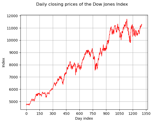
First, we load the Dow Jones dataset and plot it through time. We can see that the process is non-stationary.
full = pd.read_csv(coles.Coles().dowjones, index_col=0, parse_dates=True)
print(full[:10])
graph = ot.Graph(
    "Daily closing prices of the Dow Jones Index", "Day index", "Index", True, ""
)
# Care: to get the real period range, multiply by a factor to account for non-working days missing values!
size = len(full)
days = ot.Sample([[i] for i in range(size)])
dataDowJones = ot.Sample.BuildFromDataFrame(full)
curve = ot.Curve(days, dataDowJones)
curve.setColor("red")
graph.add(curve)
graph.setIntegerXTick(True)
view = otv.View(graph)
                       Index
Date
1995-09-11 02:00:00  4704.94
1995-09-12 02:00:00  4747.21
1995-09-13 02:00:00  4765.52
1995-09-14 02:00:00  4801.80
1995-09-15 02:00:00  4797.57
1995-09-18 02:00:00  4780.41
1995-09-19 02:00:00  4767.04
1995-09-20 02:00:00  4792.69
1995-09-21 02:00:00  4767.40
1995-09-22 02:00:00  4764.15
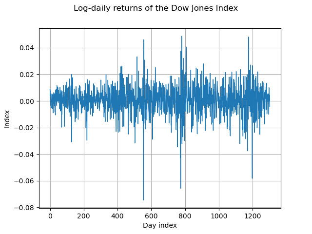
In that example, the time dependence can not be explained by trends or seasonal cycles. Many empirical studies have advised to consider the logarithms of ratios of successive observations to get an approximation to stationarity. We apply that transformation:
The resulting time series appears to be reasonably close to stationarity.
transfDataDJ = ot.Sample(
    [
        [m.log(dataDowJones[i, 0]) - m.log(dataDowJones[i - 1, 0])]
        for i in range(1, size)
    ]
)
curve = ot.Curve(days[:-1], transfDataDJ)
graph = ot.Graph(
    "Log-daily returns of the Dow Jones Index", "Day index", "Index", True, ""
)
graph.add(curve)
view = otv.View(graph)
For convenience of presentation, we rescale the data:
scalTransfDataDJ = transfDataDJ * 100.0
size = len(scalTransfDataDJ)
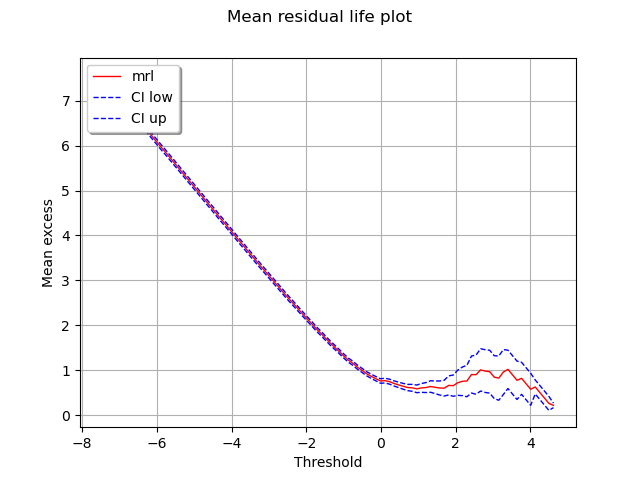
In order to select a threshold upon which the GPD model will be fitted, we draw
the mean residual life plot with approximate confidence interval.
The curve is initially linear and shows significant curvature for
. Then for
, the curve is considered as
reasonably linear when judged to confidence intervals. Hence, we
choose the threshold
. There are 37 exceedances of
.
factory = ot.GeneralizedParetoFactory()
graph = factory.drawMeanResidualLife(scalTransfDataDJ)
view = otv.View(graph)
u = 2.0
Stationary GPD modeling assuming independence in data
We first assume that the dependence between the transformed data
is negligible, so we first consider the data as
independent observations over the observation period.
We estimate the parameters of the GPD distribution modeling the excesses
above by maximizing the log-likelihood of the excesses.
result_LL = factory.buildMethodOfLikelihoodMaximizationEstimator(scalTransfDataDJ, u)
We get the fitted GPD and the estimated parameters .
fitted_GPD = result_LL.getDistribution()
desc = fitted_GPD.getParameterDescription()
param = fitted_GPD.getParameter()
print(", ".join([f"{p}: {value:.3f}" for p, value in zip(desc, param)]))
print("log-likelihood = ", result_LL.getLogLikelihood())
sigma: 0.626, xi: 0.066, u: 2.000
log-likelihood =  -22.103513585430218
We get the asymptotic distribution of the estimator .
The threshold
has not been estimated to ensure the regularity
of the model and then the asymptotic properties of the maximum likelihood
estimators. This is the reason why it appears as a Dirac distribution centered on
the chosen threshold.
In that case, the asymptotic distribution of
is normal.
parameterEstimate = result_LL.getParameterDistribution()
print("Asymptotic distribution of the estimator : ")
print(parameterEstimate)
Asymptotic distribution of the estimator :
BlockIndependentDistribution(Normal(mu = [0.625758,0.0661835], sigma = [0.1838,0.193486], R = [[  1        -0.795905 ]
 [ -0.795905  1        ]]), Dirac(point = [2]))
We get the covariance matrix and the standard deviation of
where
is deterministic.
print("Cov matrix = \n", parameterEstimate.getCovariance())
print("Standard dev = ", parameterEstimate.getStandardDeviation())
Cov matrix =
 [[  0.0337823 -0.0283045  0         ]
 [ -0.0283045  0.0374369  0         ]
 [  0          0          0         ]]
Standard dev =  [0.1838,0.193486,0]
We get the marginal confidence intervals of order 0.95 of
.
order = 0.95
for i in range(2):  # exclude u parameter (fixed)
    ci = parameterEstimate.getMarginal(i).computeBilateralConfidenceInterval(order)
    print(desc[i] + ":", ci)
sigma: [0.265518, 0.985999]
xi: [-0.313043, 0.44541]
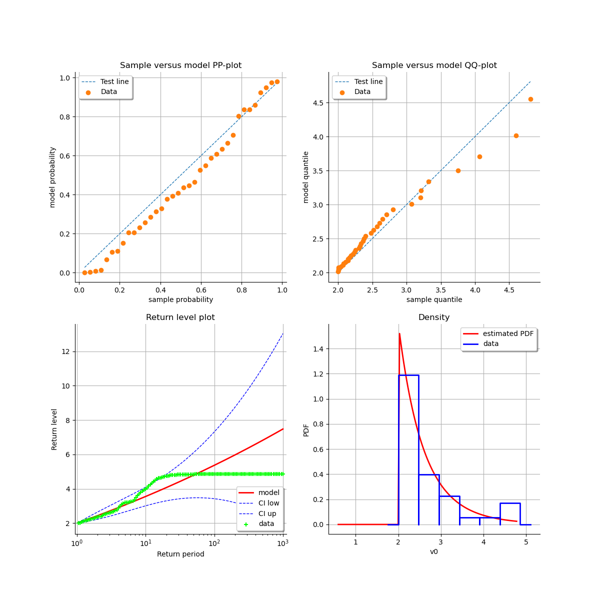
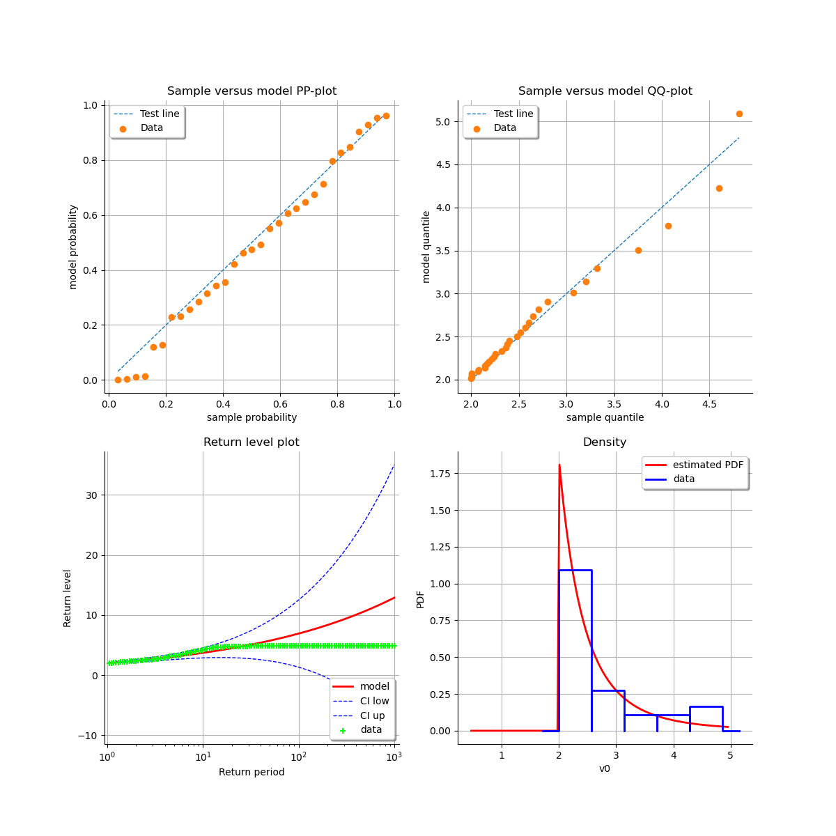
At last, we can check the quality of the inference thanks to the 4 usual diagnostic plots:
the probability-probability pot,
the quantile-quantile pot,
the return level plot,
the data histogram and the density of the fitted model.
We conclude that the goodness-of-fit in the quantile plots seems unconvincing,
even if the other plots appear to be reasonable. This is due to the fact that
the excesses can not be considered as independent: the transformed series
has a rich structure of temporal dependence.
validation = otexp.GeneralizedParetoValidation(result_LL, scalTransfDataDJ)
graph = validation.drawDiagnosticPlot()
view = otv.View(graph)
Stationary GPD modeling taking into account the dependence in data
We illustrate the fact that the excesses of the transformed series happen in groups. Hence we use the declustering method which filters the dependent observations exceeding a given threshold to obtain a set of threshold excesses that can be assumed as independent.
Consecutive exceedances of belong to the same cluster. Two distinct
clusters are separated by
consecutive observations under the
threshold. Within each cluster, we select the maximum value that will be used to
infer the GPD distribution. The cluster maxima are assumed to be independent.
On the graph, we show the clusters over the threshold
and all the maxima selected within each cluster.
It is possible to extract the data belonging to the same cluster and the
cluster maximum series.
We denote by
the number of clusters and
by
the number of exceedances above
.
part = otexp.SamplePartition(scalTransfDataDJ)
r = 3
peaks, clusters = part.getPeakOverThreshold(u, r)
nc = len(peaks)
nu = sum([1 if scalTransfDataDJ[i, 0] > u else 0 for i in range(size)])
print(f"nc={nc} nu={u} theta={nc / nu:.3f}")
graph = clusters.draw(u)
graph.setTitle(
    "Threshold exceedances and clusters by transformed Dow Jones Index series"
)
view = otv.View(graph)
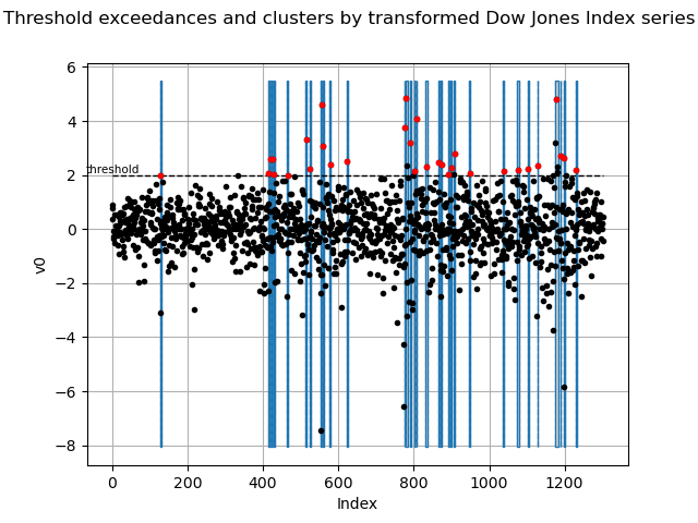
nc=32 nu=2.0 theta=0.865
We estimate a stationary GPD on the clusters maxima which are independent
with the confidence interval of each parameter.
result_LL = factory.buildMethodOfLikelihoodMaximizationEstimator(peaks, u)
sigma, xi, _ = result_LL.getParameterDistribution().getMean()
sigma_stddev, xi_stddev, _ = result_LL.getParameterDistribution().getStandardDeviation()
print(
    f"u={u} r={r} nc={nc} sigma={sigma:.2f} ({sigma_stddev:.2f}) xi={xi:.2f} ({xi_stddev:.2f})",
    end=" ",
)
u=2.0 r=3 nc=32 sigma=0.54 (0.18) xi=0.27 (0.28)
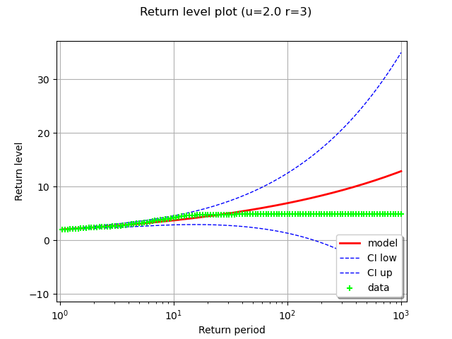
We evaluate the -year return level which corresponds to the
-observation return level, where
with
the number of observations per year. Here, we have daily observations, hence
. To calculate it, we evaluate the extremal index
which is the inverse of the mean length of the clusters,
estimated by the ratio between the number of clusters and the number
of exceedances of
.
theta = nc / nu
ny = 365
T = 100
xm_100 = factory.buildReturnLevelEstimator(result_LL, scalTransfDataDJ, T * ny, theta)
print(f"x100={xm_100.getMean()} ({xm_100.getStandardDeviation()}) theta={theta:.3f}")
x100=[12.5097] ([10.6691]) theta=0.865
We plot the return level for the new fitted model that takes into account dependence between excesses. We can see the fitted model works well. However, the large return level confidence intervals obtained for extreme return levels makes it difficult to make reliable predictions with any degree of certainty.
validation = otexp.GeneralizedParetoValidation(result_LL, peaks)
grid = validation.drawDiagnosticPlot()
rlPlot = grid.getGraph(1, 0)
rlPlot.setTitle(rlPlot.getTitle() + f" (u={u} r={r})")
view = otv.View(rlPlot)
We plot the whole series of validation graphs of the new fitted model.
view = otv.View(grid)
otv.View.ShowAll()
 OpenTURNS