Note
Go to the end to download the full example code.
Estimate tail dependence coefficients on the wave-surge data
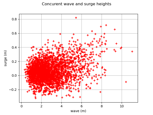
In this example we estimate the tail dependence coefficient of a bivariate sample applied to the concurrent measurements of two oceanographic variables (wave and surge heights) at a single location off south-west England. Readers should refer to [coles2001] to get more details.
First, we load the wave-surge dataset.
import openturns as ot
import openturns.viewer as otv
from openturns.usecases import coles

data = coles.Coles().wavesurge
print(data[:5])

graph = ot.Graph("Concurent wave and surge heights", "wave (m)", "surge (m)", True, "")
cloud = ot.Cloud(data)
cloud.setColor("red")
graph.add(cloud)
view = otv.View(graph)

    [ wave   surge  ]
0 : [  1.5   -0.009 ]
1 : [  1.83  -0.053 ]
2 : [  2.44  -0.024 ]
3 : [  1.68   0     ]
4 : [  1.49   0.079 ]
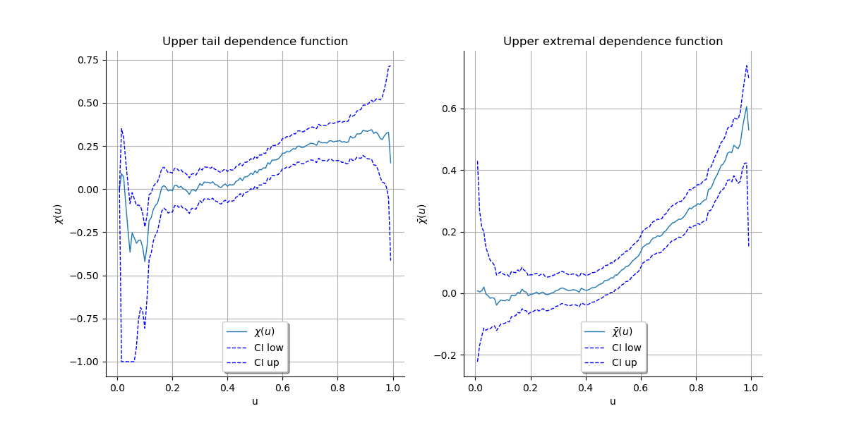
We plot the graph of the function and the graph of the function
. We conclude that both variables are asymptotially dependent
as
and that they are positively correlated as
.
We can visually deduce the upper tail dependence coefficient
and
the upper extremal dependence coefficient
.
graph1 = ot.VisualTest.DrawUpperTailDependenceFunction(data)
graph2 = ot.VisualTest.DrawUpperExtremalDependenceFunction(data)
grid = ot.GridLayout(1, 2)
grid.setGraph(0, 0, graph1)
grid.setGraph(0, 1, graph2)
view = otv.View(grid)

otv.View.ShowAll()
 OpenTURNS