Note
Go to the end to download the full example code.
Optimization using NLopt
In this example we are going to explore optimization using the interface to the NLopt library.
import openturns as ot
import openturns.viewer as viewer
from matplotlib import pylab as plt

ot.Log.Show(ot.Log.NONE)
List available algorithms
for algo in ot.NLopt.GetAlgorithmNames():
    print(algo)
AUGLAG
AUGLAG_EQ
GD_MLSL
GD_MLSL_LDS
GN_CRS2_LM
GN_DIRECT
GN_DIRECT_L
GN_DIRECT_L_NOSCAL
GN_DIRECT_L_RAND
GN_DIRECT_L_RAND_NOSCAL
GN_DIRECT_NOSCAL
GN_ESCH
GN_ISRES
GN_MLSL
GN_MLSL_LDS
GN_ORIG_DIRECT
GN_ORIG_DIRECT_L
G_MLSL
G_MLSL_LDS
LD_AUGLAG
LD_AUGLAG_EQ
LD_CCSAQ
LD_LBFGS
LD_MMA
LD_SLSQP
LD_TNEWTON
LD_TNEWTON_PRECOND
LD_TNEWTON_PRECOND_RESTART
LD_TNEWTON_RESTART
LD_VAR1
LD_VAR2
LN_AUGLAG
LN_AUGLAG_EQ
LN_BOBYQA
LN_COBYLA
LN_NELDERMEAD
LN_NEWUOA
LN_SBPLX
More details on NLopt algorithms are available here .
The optimization algorithm is instantiated from the NLopt name
algo = ot.NLopt("LD_SLSQP")
define the problem
objective = ot.SymbolicFunction(["x1", "x2"], ["100*(x2-x1^2)^2+(1-x1)^2"])
inequality_constraint = ot.SymbolicFunction(["x1", "x2"], ["x1-2*x2"])
dim = objective.getInputDimension()
bounds = ot.Interval([-3.0] * dim, [5.0] * dim)
problem = ot.OptimizationProblem(objective)
problem.setMinimization(True)
problem.setInequalityConstraint(inequality_constraint)
problem.setBounds(bounds)
solve the problem
algo.setProblem(problem)
startingPoint = [0.0] * dim
algo.setStartingPoint(startingPoint)
algo.run()
retrieve results
result = algo.getResult()
print("x^=", result.getOptimalPoint())
x^= [0.517441,0.258721]
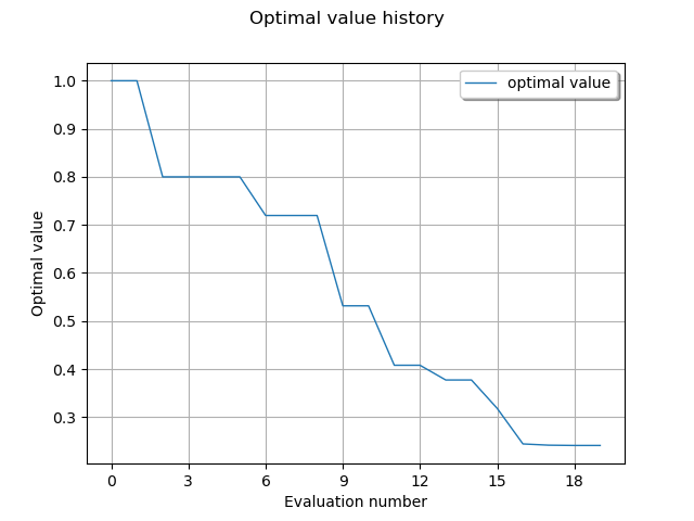
draw optimal value history
graph = result.drawOptimalValueHistory()
view = viewer.View(graph)
plt.show()

 OpenTURNS