Note
Go to the end to download the full example code.
Create a discrete Markov chain process
This example details first how to create and manipulate a discrete Markov chain.
A discrete Markov chain , where
is a process
where
discretized on the time grid
such
that:
The transition matrix of the process can be defined such that:
The library proposes to model it through the object DiscreteMarkovChain defined thanks to the origin
(which can be either deterministic or uncertain), the transition matrix
and the time grid.
import openturns as ot
import openturns.viewer as viewer
from matplotlib import pylab as plt

ot.Log.Show(ot.Log.NONE)
Define a generic function to plot matrices
def plotMatrix(matrix, texts=False, origin=None, colorbar=False, extent=None, **kwargs):
    """Generic procedure for displaying a matrix with or without text overlay and color bar"""
    res = plt.matshow(matrix, origin=origin, extent=extent, **kwargs)
    if texts:
        if extent is None:
            extent = (-0.5, matrix.getNbColumns() - 0.5, -0.5, matrix.getNbRows() - 0.5)
        x_step = (extent[1] - extent[0]) / matrix.getNbColumns()
        y_step = (extent[3] - extent[2]) / matrix.getNbRows()
        for i in range(matrix.getNbColumns()):
            for j in range(matrix.getNbRows()):
                c = round(
                    matrix[j if origin == "lower" else (matrix.getNbRows() - j - 1), i],
                    2,
                )
                plt.text(
                    i * x_step + extent[0] + x_step / 2,
                    j * y_step + extent[2] + y_step / 2,
                    str(c),
                    va="center",
                    ha="center",
                )
    if colorbar:
        plt.colorbar(res)
Define the origin
origin = ot.Dirac(0.0)
Define the transition matrix
transition = ot.SquareMatrix(
    [
        [0.1, 0.3, 0.5, 0.1],
        [0.6, 0.1, 0.2, 0.1],
        [0.4, 0.3, 0.1, 0.2],
        [0.2, 0.0, 0.1, 0.7],
    ]
)
Visualize the transition matrix
plt.matshow(transition)
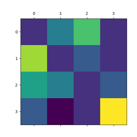
<matplotlib.image.AxesImage object at 0x7ff3e53bbb00>
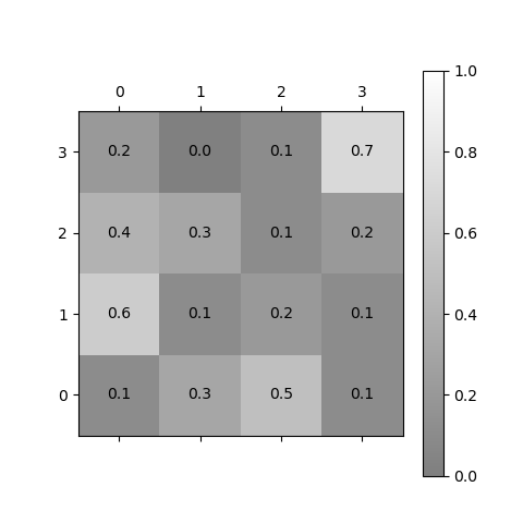
Invert axes and add texts
plotMatrix(
    transition,
    cmap="gray",
    texts=True,
    origin="lower",
    colorbar=True,
    alpha=0.5,
    vmin=0,
    vmax=1,
)
Define an 1-d mesh
tgrid = ot.RegularGrid(0.0, 1.0, 50)
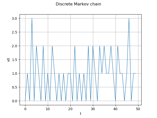
Markov chain definition and realization
process = ot.DiscreteMarkovChain(origin, transition, tgrid)
real = process.getRealization()
graph = real.drawMarginal(0)
graph.setTitle("Discrete Markov chain")
view = viewer.View(graph)
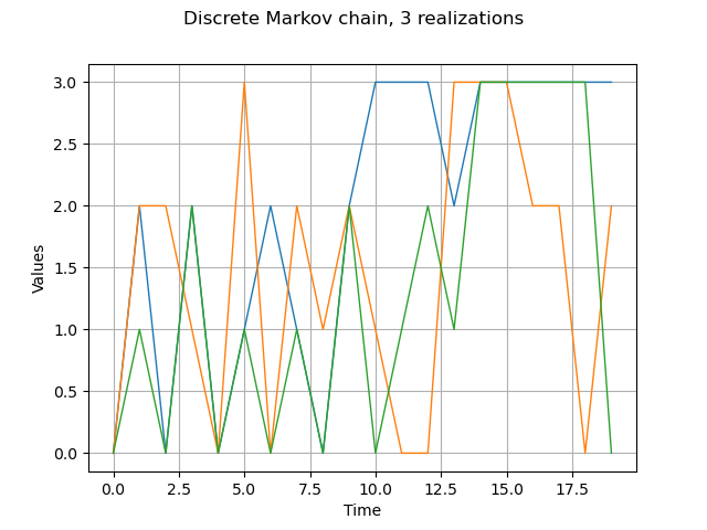
Get several realizations
process.setTimeGrid(ot.RegularGrid(0.0, 1.0, 20))
reals = process.getSample(3)
graph = reals.drawMarginal(0)
graph.setTitle("Discrete Markov chain, 3 realizations")
view = viewer.View(graph)
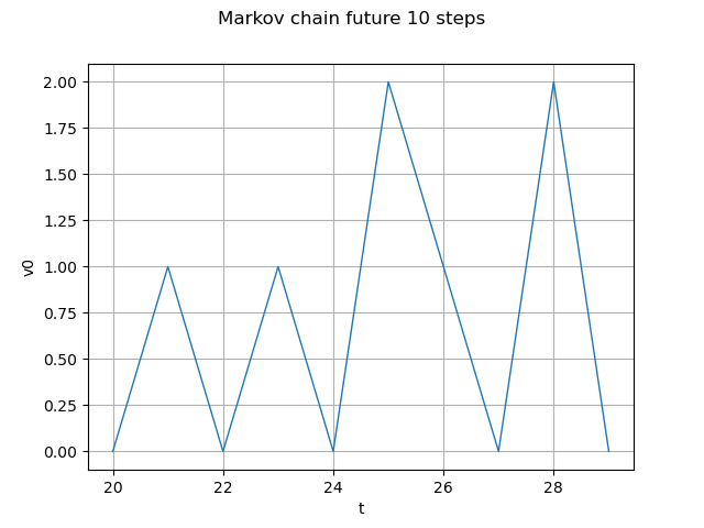
Markov chain future 10 steps
future = process.getFuture(10)
graph = future.drawMarginal(0)
graph.setTitle("Markov chain future 10 steps")
view = viewer.View(graph)
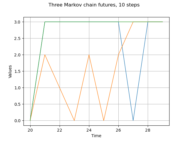
Markov chain 3 different futures
futures = process.getFuture(10, 3)
graph = futures.drawMarginal(0)
graph.setTitle("Three Markov chain futures, 10 steps")
view = viewer.View(graph)
plt.show()
 OpenTURNS