QQ-plot
The Quantile - Quantile - Plot (QQ Plot) enables to validate whether two given samples of data are drawn from the same continuous distribution of dimension 1.
We denote by
and
two given samples of dimension 1.
A QQ-Plot is based on the comparison of some empirical quantiles. Let
be the quantile of order
of the distribution
, with
. It is defined by:
The empirical quantile of order built on the sample is defined by:
where denotes the integral part of
and
is the sample sorted in ascended order:
Thus, the smallest value of the sample
is an estimate
of the
-quantile where
, for
.
The QQ-plot draws the couples of empirical quantiles of the same order from both samples:
.
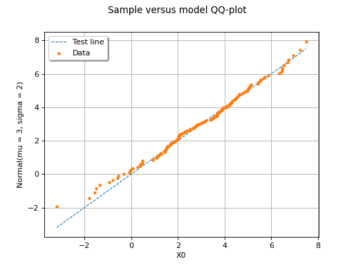
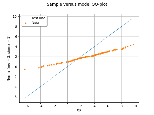
If both samples follow the same distribution, then the points should be close to the diagonal.
The following figure illustrates a QQ-plot with two
samples of size . In this example, the
points remain close to the diagonal and the hypothesis
“Both samples are drawn from the same distribution” does not seem false,
even if a more quantitative analysis should be
carried out to confirm this.
(Source code, png)

(Source code, png)

In this second example, the two samples clearly arise from two different distributions.
 OpenTURNS