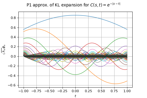
KarhunenLoeveP1Algorithm
(Source code, png)

- class KarhunenLoeveP1Algorithm(*args)
Computation of Karhunen-Loeve decomposition using P1 approximation.
- Parameters:
- mesh
Mesh The mesh
that discretizes the domain
.
- covariance
CovarianceModel The covariance function to decompose.
- sfloat,
The threshold used to select the most significant eigenmodes, defined in
KarhunenLoeveAlgorithm.
- mesh
Notes
The Karhunen-Loeve
algorithm solves the Fredholm problem associated to the covariance function
: see
KarhunenLoeveAlgorithmfor the notations.The Karhunen-Loeve
approximation uses the
functional basis
where
are the basis functions of the
finite element space associated to
, whose vertices are
.
The covariance function
is approximated by its
approximation
on
:
The Galerkin approach and the collocation one are equivalent in the
approach and both lead to the following formulation:
where
with
,
.
Though the eigenvalues computation is performed by LAPACK by default, several other solvers can be used. The solver to use must be specified by setting the
KarhunenLoeveP1Algorithm-EigenvaluesSolverkey inResourceMap. Some solvers set limits to the number of eigenvalues they can compute with regards to the size of the problem. The following table summarizes the supported solvers and their maximum number of eigenvalues for a problem of size:
Solver
ResourceMap key
Maximum EV number
Lapack
LAPACK
Spectra
SPECTRA
For large dimension problems, it can be useful to generate the covariance matrix of the problem as a
HMatrixinstead of a standard dense matrix. In this case, one can set theKarhunenLoeveP1Algorithm-CovarianceMatrixStoragekey inResourceMaptoHMAT(instead ofDENSE).Examples
Create a Karhunen-Loeve P1 algorithm:
>>> import openturns as ot
>>> mesh = ot.IntervalMesher([10]*2).build(ot.Interval([-1.0]*2, [1.0]*2))
>>> s = 0.01
>>> model = ot.AbsoluteExponential([1.0]*2)
>>> algorithm = ot.KarhunenLoeveP1Algorithm(mesh, model, s)
Run it!
>>> algorithm.run()
>>> result = algorithm.getResult()
Methods
Accessor to the object's name.
Accessor to the covariance model.
getMesh()Accessor to the mesh.
getName()Accessor to the object's name.
Accessor to number of modes to compute.
Get the result structure.
Accessor to the threshold used to select the most significant eigenmodes.
hasName()Test if the object is named.
run()Computation of the eigenvalues and eigenfunctions values at nodes.
setCovarianceModel(covariance)Accessor to the covariance model.
setName(name)Accessor to the object's name.
setNbModes(nbModes)Accessor to the maximum number of modes to compute.
setThreshold(threshold)Accessor to the limit ratio on eigenvalues.
- __init__(*args)
- getClassName()
Accessor to the object’s name.
- Returns:
- class_namestr
The object class name (object.__class__.__name__).
- getCovarianceModel()
Accessor to the covariance model.
- Returns:
- covModel
CovarianceModel The covariance model.
- covModel
- getName()
Accessor to the object’s name.
- Returns:
- namestr
The name of the object.
- getNbModes()
Accessor to number of modes to compute.
- Returns:
- nint
The maximum number of modes to compute. The actual number of modes also depends on the threshold criterion.
- getResult()
Get the result structure.
- Returns:
- resKL
KarhunenLoeveResult The structure containing all the results of the Fredholm problem.
- resKL
Notes
The structure contains all the results of the Fredholm problem.
- getThreshold()
Accessor to the threshold used to select the most significant eigenmodes.
- Returns:
- sfloat, positive
The threshold
.
Notes
OpenTURNS truncates the sequence
at the index
defined in (3).
- hasName()
Test if the object is named.
- Returns:
- hasNamebool
True if the name is not empty.
- run()
Computation of the eigenvalues and eigenfunctions values at nodes.
Notes
Runs the algorithm and creates the result structure
KarhunenLoeveResult.
- setCovarianceModel(covariance)
Accessor to the covariance model.
- Parameters:
- covModel
CovarianceModel The covariance model.
- covModel
- setName(name)
Accessor to the object’s name.
- Parameters:
- namestr
The name of the object.
- setNbModes(nbModes)
Accessor to the maximum number of modes to compute.
- Parameters:
- nint
The maximum number of modes to compute. The actual number of modes also depends on the threshold criterion.
 OpenTURNS
