Note
Go to the end to download the full example code.
Kriging : draw covariance models
import openturns as ot
import openturns.viewer as otv
from matplotlib import pylab as plt
import pylab as pl
Abstract
Gaussian processes are a common fixture in UQ. They are defined by their covariance function and the library implements several of them. In this example we plot covariance functions and modify their parameters for two families of models: the generalized exponential model and the Matérn models.
For visualization sake, we limit ourselves to the dimension 1.
dimension = 1
We set the lower bound to zero for stationary kernels
ot.ResourceMap.SetAsScalar("CovarianceModel-DefaultTMin", 0.0)
The generalized exponential model
The GeneralizedExponential class implements a generalized exponential with a
parameter exponent. The case
is the standard exponential model
while
is the squared exponential.
Various parameters p and a fixed correlation length of 0.1
In this part we set the correlation length to and study three different models
with parameters
,
and
and trajectories from Gaussian processes
based on these models.
We define the generalized exponential model :
covarianceModel = ot.GeneralizedExponential([0.1], 0.25)
We define the generalized exponential model :
covarianceModel2 = ot.GeneralizedExponential([0.1], 1.0)
We define the generalized exponential model :
covarianceModel3 = ot.GeneralizedExponential([0.1], 2.0)
We draw the covariance models :
graphModel = covarianceModel.draw()
graphModel.add(covarianceModel2.draw())
graphModel.add(covarianceModel3.draw())
graphModel.setColors(["green", "orange", "blue"])
graphModel.setXTitle(r"$\tau = \|s-t\|$")
graphModel.setYTitle(r"$C(\tau)$")
graphModel.setLegends([r"$p = 0.25$", r"$p = 1$", r"$p = 2$"])
For each covariance model we build a Gaussian process and generate a random trajectory of
on .
We first build a discretization of this interval with a regular grid with step 0.01.
xmin = -1.0
step = 0.01
n = 200
grid1D = ot.RegularGrid(xmin, step, n + 1)
nbTrajectories = 1
We define the first Gaussian process and its trajectory :
process = ot.GaussianProcess(covarianceModel, grid1D)
sample = process.getSample(nbTrajectories)
then the second one and its trajectory :
process2 = ot.GaussianProcess(covarianceModel2, grid1D)
sample2 = process2.getSample(nbTrajectories)
and finally the third one and its trajectory :
process3 = ot.GaussianProcess(covarianceModel3, grid1D)
sample3 = process3.getSample(nbTrajectories)
We draw the trajectories :
graphTraj = sample.drawMarginal(0)
graphTraj.add(sample2.drawMarginal(0))
graphTraj.add(sample3.drawMarginal(0))
graphTraj.setXTitle(r"$x$")
graphTraj.setYTitle(r"$GP_{\nu}(x)$")
graphTraj.setTitle("Random realization from the covariance model")
graphTraj.setColors(["green", "orange", "blue"])
graphTraj.setLegends([r"$p = 0.25$", r"$p = 1$", r"$p = 2$"])
We present each covariance model and the corresponding trajectory side by side.
fig = pl.figure(figsize=(12, 4))
ax_pdf = fig.add_subplot(1, 2, 1)
_ = otv.View(graphModel, figure=fig, axes=[ax_pdf])
ax_cdf = fig.add_subplot(1, 2, 2)
_ = otv.View(graphTraj, figure=fig, axes=[ax_cdf])
_ = fig.suptitle(r"Generalized Exponential Model : influence of the p parameter")
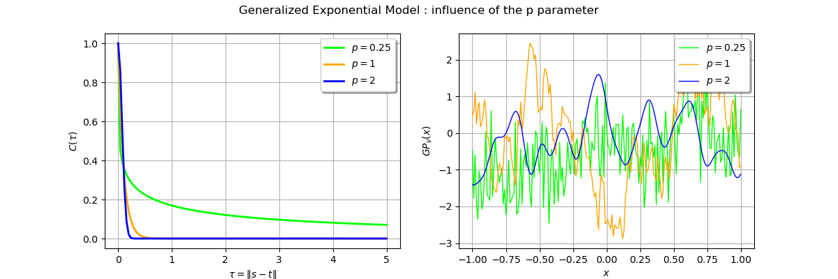
The blue trajectory corresponding to the parameter is smooth as expected as compared with
the
process which is less regular.
The exponential model ( )
)
In the case of the exponential model () we show the influence of the correlation length on
the trajectories.
with correlation length :
covarianceModel = ot.GeneralizedExponential([0.01], 1.0)
with correlation length :
covarianceModel2 = ot.GeneralizedExponential([0.1], 1.0)
with correlation length
covarianceModel3 = ot.GeneralizedExponential([1.0], 1.0)
We draw the covariance models :
graphModel = covarianceModel.draw()
graphModel.add(covarianceModel2.draw())
graphModel.add(covarianceModel3.draw())
graphModel.setColors(["green", "orange", "blue"])
graphModel.setXTitle(r"$\tau = \|s-t\|$")
graphModel.setYTitle(r"$C(\tau)$")
graphModel.setLegends([r"$\theta = 0.01$", r"$\theta = 0.1$", r"$\theta = 1$"])
For each covariance model we build a Gaussian process and generate a random trajectory of
on .
We first build a discretization of this interval with a regular grid with step 0.01.
xmin = -1.0
step = 0.01
n = 200
grid1D = ot.RegularGrid(xmin, step, n + 1)
nbTrajectories = 1
We define the first Gaussian process and its trajectory :
process = ot.GaussianProcess(covarianceModel, grid1D)
sample = process.getSample(nbTrajectories)
then the second one and its trajectory :
process2 = ot.GaussianProcess(covarianceModel2, grid1D)
sample2 = process2.getSample(nbTrajectories)
and finally the third one and its trajectory :
process3 = ot.GaussianProcess(covarianceModel3, grid1D)
sample3 = process3.getSample(nbTrajectories)
We draw the trajectories :
graphTraj = sample.drawMarginal(0)
graphTraj.add(sample2.drawMarginal(0))
graphTraj.add(sample3.drawMarginal(0))
graphTraj.setXTitle(r"$x$")
graphTraj.setYTitle(r"$GP_{\theta}(x)$")
graphTraj.setTitle("Random realization from the covariance model")
graphTraj.setColors(["green", "orange", "blue"])
graphTraj.setLegends([r"$\theta = 0.01$", r"$\theta = 0.1$", r"$\theta = 1$"])
We present each covariance model and the corresponding tracjectory side by side.
fig = pl.figure(figsize=(12, 4))
ax_pdf = fig.add_subplot(1, 2, 1)
_ = otv.View(graphModel, figure=fig, axes=[ax_pdf])
ax_cdf = fig.add_subplot(1, 2, 2)
_ = otv.View(graphTraj, figure=fig, axes=[ax_cdf])
_ = fig.suptitle(r"Exponential Model : influence of correlation length $\theta$")
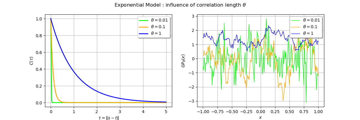
We observe a smoother trajectory with a high correlation value.
The squared exponential ( )
)
In the case of the squared exponential model () we show the influence of the correlation length on
the trajectories.
with correlation length :
covarianceModel = ot.GeneralizedExponential([0.01], 2.0)
with correlation length :
covarianceModel2 = ot.GeneralizedExponential([0.1], 2.0)
with correlation length
covarianceModel3 = ot.GeneralizedExponential([1.0], 2.0)
We draw the covariance models :
graphModel = covarianceModel.draw()
graphModel.add(covarianceModel2.draw())
graphModel.add(covarianceModel3.draw())
graphModel.setColors(["green", "orange", "blue"])
graphModel.setXTitle(r"$\tau = \|s-t\|$")
graphModel.setYTitle(r"$C(\tau)$")
graphModel.setLegends([r"$\theta = 0.01$", r"$\theta = 0.1$", r"$\theta = 1$"])
For each covariance model we build a Gaussian process and generate a random trajectory of
on .
We first build a discretization of this interval with a regular grid with step 0.01.
xmin = -1.0
step = 0.01
n = 200
grid1D = ot.RegularGrid(xmin, step, n + 1)
nbTrajectories = 1
We define the first Gaussian process and its trajectory :
process = ot.GaussianProcess(covarianceModel, grid1D)
sample = process.getSample(nbTrajectories)
then the second one and its trajectory :
process2 = ot.GaussianProcess(covarianceModel2, grid1D)
sample2 = process2.getSample(nbTrajectories)
and finally the third one and its trajectory :
process3 = ot.GaussianProcess(covarianceModel3, grid1D)
sample3 = process3.getSample(nbTrajectories)
We draw the trajectories :
graphTraj = sample.drawMarginal(0)
graphTraj.add(sample2.drawMarginal(0))
graphTraj.add(sample3.drawMarginal(0))
graphTraj.setXTitle(r"$x$")
graphTraj.setYTitle(r"$GP_{\theta}(x)$")
graphTraj.setTitle("Random realization from the covariance model")
graphTraj.setColors(["green", "orange", "blue"])
graphTraj.setLegends([r"$\theta = 0.01$", r"$\theta = 0.1$", r"$\theta = 1$"])
We present each covariance model and the corresponding tracjectory side by side.
fig = pl.figure(figsize=(12, 4))
ax_pdf = fig.add_subplot(1, 2, 1)
_ = otv.View(graphModel, figure=fig, axes=[ax_pdf])
ax_cdf = fig.add_subplot(1, 2, 2)
_ = otv.View(graphTraj, figure=fig, axes=[ax_cdf])
_ = fig.suptitle(
    r"Squared exponential model : influence of correlation length $\theta$"
)
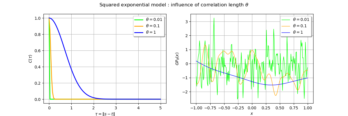
Except for very small values of the correlation length, trajectories are usually smooth. It is the main effect of the squared exponential model which leads to smooth processes.
The Matérn covariance model
The MaternModel class implements the Matern model of parameter .
This parameter controls the smoothness of the process : for any
the
process is
times continuously differentiable.
Influence of the regularity
In this paragraph we represent three models with different regularity and generate the
corresponding random trajectories. We shall use ,
and
and observe the regularity.
We define the Matern model :
covarianceModel = ot.MaternModel([1.0], 0.5)
We define the Matern model :
covarianceModel2 = ot.MaternModel([1.0], 1.5)
We define the Matern model :
covarianceModel3 = ot.MaternModel([1.0], 2.5)
We draw the covariance models :
graphModel = covarianceModel.draw()
graphModel.add(covarianceModel2.draw())
graphModel.add(covarianceModel3.draw())
graphModel.setColors(["green", "orange", "blue"])
graphModel.setXTitle(r"$\tau = \|s-t\|$")
graphModel.setYTitle(r"$C(\tau)$")
graphModel.setLegends([r"$\nu = 1/2$", r"$\nu = 3/2$", r"$\nu = 5/2$"])
For each covariance model we build a Gaussian process and generate a random trajectory of
on .
We first build a discretization of this interval with a regular grid with step 0.001.
xmin = -5.0
step = 0.01
n = 1000
grid1D = ot.RegularGrid(xmin, step, n + 1)
nbTrajectories = 1
We define the first Gaussian process and its trajectory :
process = ot.GaussianProcess(covarianceModel, grid1D)
sample = process.getSample(nbTrajectories)
then the second one and its trajectory :
process2 = ot.GaussianProcess(covarianceModel2, grid1D)
sample2 = process2.getSample(nbTrajectories)
and finally the third one and its trajectory :
process3 = ot.GaussianProcess(covarianceModel3, grid1D)
sample3 = process3.getSample(nbTrajectories)
We draw the trajectories :
graphTraj = sample.drawMarginal(0)
graphTraj.add(sample2.drawMarginal(0))
graphTraj.add(sample3.drawMarginal(0))
graphTraj.setXTitle(r"$x$")
graphTraj.setYTitle(r"$GP_{\nu}(x)$")
graphTraj.setTitle("Random realization from the covariance model")
graphTraj.setColors(["green", "orange", "blue"])
graphTraj.setLegends([r"$\nu = 1/2$", r"$\nu = 3/2$", r"$\nu = 5/2$"])
We present each covariance model and the corresponding tracjectory side by side.
fig = pl.figure(figsize=(12, 4))
ax_pdf = fig.add_subplot(1, 2, 1)
_ = otv.View(graphModel, figure=fig, axes=[ax_pdf])
ax_cdf = fig.add_subplot(1, 2, 2)
_ = otv.View(graphTraj, figure=fig, axes=[ax_cdf])
_ = fig.suptitle(r"Matern model : influence of the regularity $\nu$ parameter")
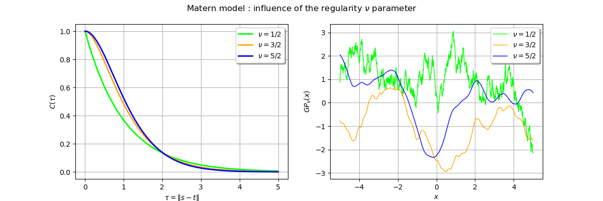
The red trajectory is the least regular () as it is only continuous. We see that the
the blue trajectory is more smooth as expected.
Variation of the correlation length
In this paragraph we fix the regularity by choosing so we expect a continuously
differentiable realization.
We then use three different correlation lengths
,
and
and observe the impact on realizations of Gaussian processes based on these
covariance models.
We define the Matern model with :
covarianceModel = ot.MaternModel([0.01], 1.5)
We define the Matern model with :
covarianceModel2 = ot.MaternModel([0.1], 1.5)
We define the Matern model with :
covarianceModel3 = ot.MaternModel([1.0], 1.5)
We draw the covariance models :
graphModel = covarianceModel.draw()
graphModel.add(covarianceModel2.draw())
graphModel.add(covarianceModel3.draw())
graphModel.setColors(["green", "orange", "blue"])
graphModel.setXTitle(r"$\tau = \|s-t\|$")
graphModel.setYTitle(r"$C(\tau)$")
graphModel.setTitle("Matern covariance model with \nu = 3/2")
graphModel.setLegends([r"$\theta = 0.01$", r"$\theta = 0.1$", r"$\theta = 1.0$"])
For each covariance model we build a Gaussian process and generate a random trajectory of
on .
We build a discretization of this interval with a regular grid with step 0.01.
xmin = -1.0
step = 0.01
n = 200
grid1D = ot.RegularGrid(xmin, step, n + 1)
nbTrajectories = 1
We define the first Gaussian process and its trajectory :
process = ot.GaussianProcess(covarianceModel, grid1D)
sample = process.getSample(nbTrajectories)
then the second process :
process2 = ot.GaussianProcess(covarianceModel2, grid1D)
sample2 = process2.getSample(nbTrajectories)
and the third one :
process3 = ot.GaussianProcess(covarianceModel3, grid1D)
sample3 = process3.getSample(nbTrajectories)
We draw the trajectories :
graphTraj = sample.drawMarginal(0)
graphTraj.add(sample2.drawMarginal(0))
graphTraj.add(sample3.drawMarginal(0))
graphTraj.setXTitle(r"$x$")
graphTraj.setYTitle(r"$GP_{\theta}(x)$")
graphTraj.setColors(["green", "orange", "blue"])
graphTraj.setLegends([r"$\theta = 0.01$", r"$\theta = 0.1$", r"$\theta = 1.0$"])
We present each covariance model and the corresponding tracjectory side by side.
fig = pl.figure(figsize=(12, 4))
ax_pdf = fig.add_subplot(1, 2, 1)
_ = otv.View(graphModel, figure=fig, axes=[ax_pdf])
ax_cdf = fig.add_subplot(1, 2, 2)
_ = otv.View(graphTraj, figure=fig, axes=[ax_cdf])
_ = fig.suptitle("The Matern model : variation of the correlation length")
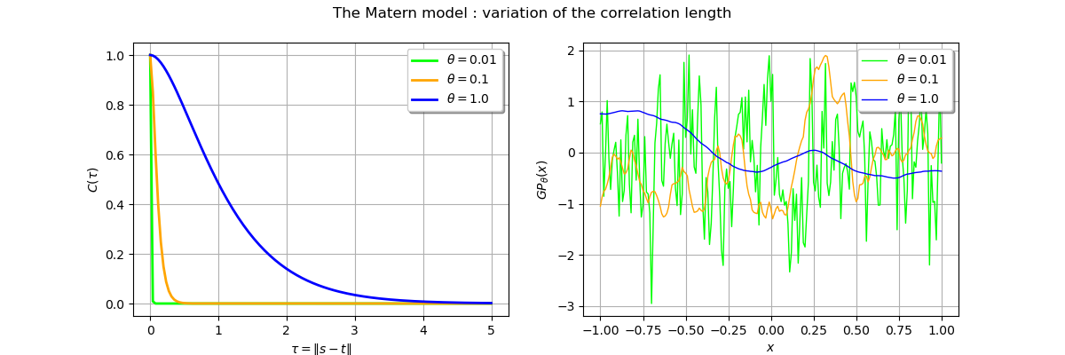
From the previous figure we see that the trajectory of the Gaussian process is smoother with large correlation length.
Display figures
plt.show()
Reset default settings
ot.ResourceMap.Reload()
 OpenTURNS