Validate a polynomial chaos

In this example, we show how to perform the validation plot of a polynomial chaos for the Ishigami function.

from openturns.usecases import ishigami_function
import openturns as ot
import openturns.viewer as viewer
from matplotlib import pylab as plt

ot.Log.Show(ot.Log.NONE)

Model description

We load the Ishigami test function from the usecases module :

im = ishigami_function.IshigamiModel()

The model contains the input distribution in im.inputDistribution and the Ishigami function in im.model. We also have access to the input variable names with

input_names = im.inputDistribution.getDescription()

N = 100
inputTrain = im.inputDistribution.getSample(N)
outputTrain = im.model(inputTrain)

Create the chaos

We could use only the input and output training samples: in this case, the distribution of the input sample is computed by selecting the best distribution that fits the data.

chaosalgo = ot.FunctionalChaosAlgorithm(inputTrain, outputTrain)

Since the input distribution is known in our particular case, we instead create the multivariate basis from the distribution, that is three independent variables , and .

multivariateBasis = ot.OrthogonalProductPolynomialFactory([im.X1, im.X2, im.X3])
totalDegree = 8
enumfunc = multivariateBasis.getEnumerateFunction()
basisSize = enumfunc.getBasisSizeFromTotalDegree(totalDegree)
adaptiveStrategy = ot.FixedStrategy(multivariateBasis, basisSize)

selectionAlgorithm = ot.LeastSquaresMetaModelSelectionFactory()
projectionStrategy = ot.LeastSquaresStrategy(
    inputTrain, outputTrain, selectionAlgorithm
)

chaosalgo = ot.FunctionalChaosAlgorithm(
    inputTrain, outputTrain, im.inputDistribution, adaptiveStrategy, projectionStrategy
)

chaosalgo.run()
result = chaosalgo.getResult()
metamodel = result.getMetaModel()

Validation of the metamodel

In order to validate the metamodel, we generate a test sample.

n_valid = 1000
inputTest = im.inputDistribution.getSample(n_valid)
outputTest = im.model(inputTest)
metamodelPredictions = metamodel(inputTest)
val = ot.MetaModelValidation(outputTest, metamodelPredictions)
r2Score = val.computeR2Score()[0]
r2Score

0.9992294812153686

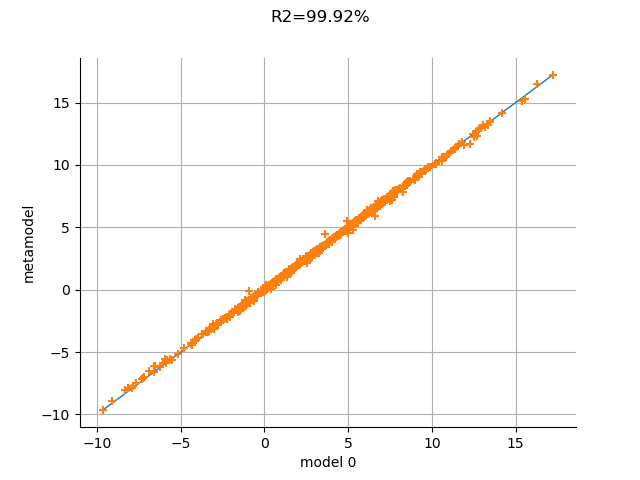
The is very close to 1: the metamodel seems very accurate.

graph = val.drawValidation()
graph.setTitle("R2=%.2f%%" % (r2Score * 100))
view = viewer.View(graph)
plt.show()

The metamodel has a good predictivity, since the points are almost on the first diagonal.