Axial stressed beam : comparing different methods to estimate a probability

In this example, we compare four methods to estimate the probability in the axial stressed beam example :

• Monte-Carlo simulation,

• FORM,

• directional sampling,

• importance sampling with FORM design point: FORM-IS.

Define the model

import numpy as np
from openturns.usecases import stressed_beam

import openturns as ot
import openturns.viewer as viewer

ot.Log.Show(ot.Log.NONE)

We load the model from the usecases module :

sm = stressed_beam.AxialStressedBeam()

The limit state function is defined in the model field of the data class :

limitStateFunction = sm.model

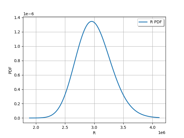
The probabilistic model of the axial stressed beam is defined in the data class. We get the first marginal and draw it :

R_dist = sm.distribution_R
graph = R_dist.drawPDF()
view = viewer.View(graph)

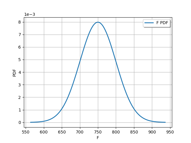
We get the second marginal and draw it :

F_dist = sm.distribution_F
graph = F_dist.drawPDF()
view = viewer.View(graph)

These independent marginals define the joint distribution of the input parameters :

myDistribution = sm.distribution

We create a RandomVector from the Distribution, then a composite random vector. Finally, we create a ThresholdEvent from this RandomVector.

inputRandomVector = ot.RandomVector(myDistribution)
outputRandomVector = ot.CompositeRandomVector(limitStateFunction, inputRandomVector)
myEvent = ot.ThresholdEvent(outputRandomVector, ot.Less(), 0.0)

Using Monte Carlo simulations

cv = 0.05
NbSim = 100000

experiment = ot.MonteCarloExperiment()
algoMC = ot.ProbabilitySimulationAlgorithm(myEvent, experiment)
algoMC.setMaximumOuterSampling(NbSim)
algoMC.setBlockSize(1)
algoMC.setMaximumCoefficientOfVariation(cv)

For statistics about the algorithm

initialNumberOfCall = limitStateFunction.getEvaluationCallsNumber()

Perform the analysis.

algoMC.run()

result = algoMC.getResult()
probabilityMonteCarlo = result.getProbabilityEstimate()
numberOfFunctionEvaluationsMonteCarlo = (
    limitStateFunction.getEvaluationCallsNumber() - initialNumberOfCall
)
print("Number of calls to the limit state =", numberOfFunctionEvaluationsMonteCarlo)
print("Pf = ", probabilityMonteCarlo)
print("CV =", result.getCoefficientOfVariation())

Number of calls to the limit state = 12927
Pf =  0.03001469791908405
CV = 0.049999621186217445

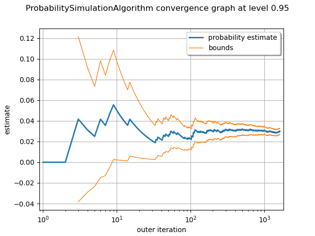
graph = algoMC.drawProbabilityConvergence()
graph.setLogScale(ot.GraphImplementation.LOGX)
view = viewer.View(graph)

Using LHS simulation

experiment = ot.LHSExperiment()
experiment.setAlwaysShuffle(True)
algo = ot.ProbabilitySimulationAlgorithm(myEvent, experiment)
algo.setMaximumOuterSampling(NbSim)
algo.setBlockSize(1)
algo.setMaximumCoefficientOfVariation(cv)

For statistics about the algorithm

initialNumberOfCall = limitStateFunction.getEvaluationCallsNumber()

Perform the analysis.

algo.run()

resultLHS = algo.getResult()

numberOfFunctionEvaluationsLHS = (
    limitStateFunction.getEvaluationCallsNumber() - initialNumberOfCall
)
probabilityLHS = result.getProbabilityEstimate()
print("Number of calls to the limit state =", numberOfFunctionEvaluationsLHS)
print("Pf = ", probabilityLHS)
print("CV =", result.getCoefficientOfVariation())

Number of calls to the limit state = 13532
Pf =  0.03001469791908405
CV = 0.049999621186217445

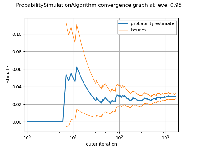
graph = algo.drawProbabilityConvergence()
graph.setLogScale(ot.GraphImplementation.LOGX)
view = viewer.View(graph)

Using FORM analysis

We create a NearestPoint algorithm

algoOptim = ot.AbdoRackwitz()
# Resolution options:
eps = 1e-3
algoOptim.setMaximumCallsNumber(1000)
algoOptim.setMaximumAbsoluteError(eps)
algoOptim.setMaximumRelativeError(eps)
algoOptim.setMaximumResidualError(eps)
algoOptim.setMaximumConstraintError(eps)

For statistics about the algorithm

initialNumberOfCall = limitStateFunction.getEvaluationCallsNumber()

We create a FORM algorithm. The first parameter is a NearestPointAlgorithm. The second parameter is an event. The third parameter is a starting point for the design point research.

algoFORM = ot.FORM(algoOptim, myEvent, myDistribution.getMean())

Perform the analysis.

algoFORM.run()

resultFORM = algoFORM.getResult()
numberOfFunctionEvaluationsFORM = (
    limitStateFunction.getEvaluationCallsNumber() - initialNumberOfCall
)
probabilityFORM = resultFORM.getEventProbability()
print("Number of calls to the limit state =", numberOfFunctionEvaluationsFORM)
print("Pf =", probabilityFORM)

Number of calls to the limit state = 7
Pf = 0.029982795362833412

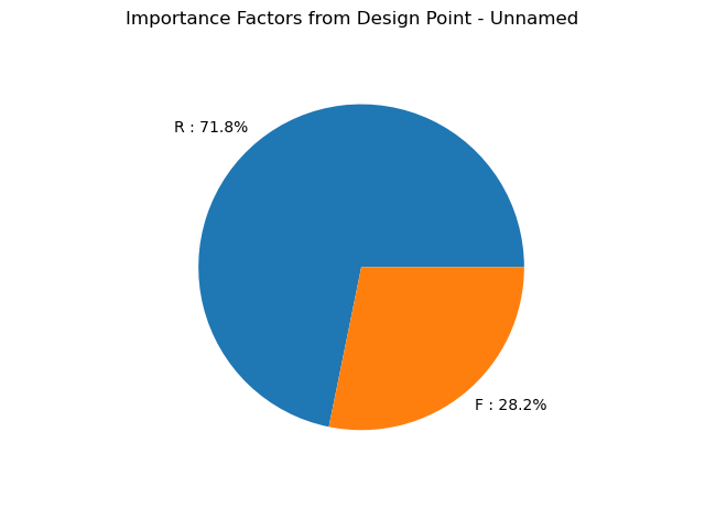
graph = resultFORM.drawImportanceFactors()
view = viewer.View(graph)

Using Directional sampling

Resolution options:

cv = 0.05
NbSim = 10000

algoDS = ot.DirectionalSampling(myEvent)
algoDS.setMaximumOuterSampling(NbSim)
algoDS.setBlockSize(1)
algoDS.setMaximumCoefficientOfVariation(cv)

For statistics about the algorithm

initialNumberOfCall = limitStateFunction.getEvaluationCallsNumber()

Perform the analysis.

algoDS.run()

result = algoDS.getResult()
probabilityDirectionalSampling = result.getProbabilityEstimate()
numberOfFunctionEvaluationsDirectionalSampling = (
    limitStateFunction.getEvaluationCallsNumber() - initialNumberOfCall
)
print(
    "Number of calls to the limit state =",
    numberOfFunctionEvaluationsDirectionalSampling,
)
print("Pf = ", probabilityDirectionalSampling)
print("CV =", result.getCoefficientOfVariation())

Number of calls to the limit state = 9479
Pf =  0.02874805526680341
CV = 0.04988071645434962

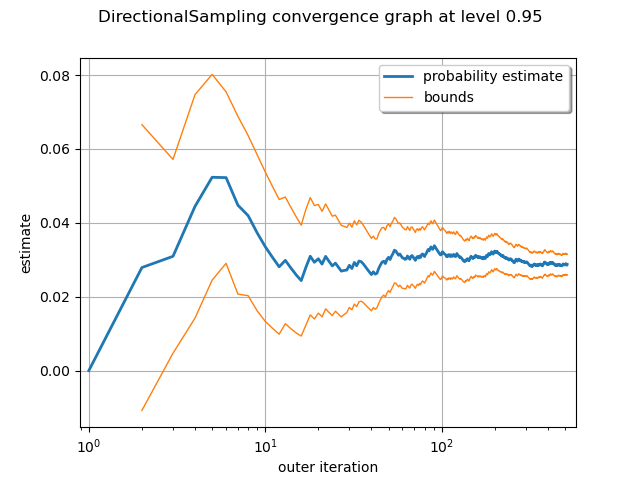
graph = algoDS.drawProbabilityConvergence()
graph.setLogScale(ot.GraphImplementation.LOGX)
view = viewer.View(graph)

Using importance sampling with FORM design point: FORM-IS

The getStandardSpaceDesignPoint method returns the design point in the U-space.

standardSpaceDesignPoint = resultFORM.getStandardSpaceDesignPoint()
standardSpaceDesignPoint

class=Point name=Standard Space Design Point dimension=2 values=[-1.59396,0.99882]

The key point is to define the importance distribution in the U-space. To define it, we use a multivariate standard Gaussian and configure it so that the center is equal to the design point in the U-space.

dimension = myDistribution.getDimension()
dimension

2

myImportance = ot.Normal(dimension)
myImportance.setMu(standardSpaceDesignPoint)
myImportance

Normal

• name=Normal
• dimension=2
• weight=1
• range=]-inf (-9.24458), (6.05667) +inf[ ]-inf (-6.65181), (8.64945) +inf[
• description=[X0,X1]
• isParallel=true
• isCopula=false

Create the design of experiment corresponding to importance sampling. This generates a WeightedExperiment with weights corresponding to the importance distribution.

experiment = ot.ImportanceSamplingExperiment(myImportance)

Create the standard event corresponding to the event. This transforms the original problem into the U-space, with Gaussian independent marginals.

standardEvent = ot.StandardEvent(myEvent)

We then create the simulation algorithm.

algo = ot.ProbabilitySimulationAlgorithm(standardEvent, experiment)
algo.setMaximumCoefficientOfVariation(cv)
algo.setMaximumOuterSampling(40000)

For statistics about the algorithm

initialNumberOfCall = limitStateFunction.getEvaluationCallsNumber()

algo.run()

retrieve results

result = algo.getResult()
probabilityFORMIS = result.getProbabilityEstimate()
numberOfFunctionEvaluationsFORMIS = (
    limitStateFunction.getEvaluationCallsNumber() - initialNumberOfCall
)
print("Number of calls to the limit state =", numberOfFunctionEvaluationsFORMIS)
print("Pf = ", probabilityFORMIS)
print("CV =", result.getCoefficientOfVariation())

Number of calls to the limit state = 891
Pf =  0.030668150809484762
CV = 0.04999634278115516

Conclusion

We now compare the different methods in terms of accuracy and speed.

The following function computes the number of correct base-10 digits in the computed result compared to the exact result.

def computeLogRelativeError(exact, computed):
    logRelativeError = -np.log10(abs(exact - computed) / abs(exact))
    return logRelativeError

The following function prints the results.

def printMethodSummary(name, computedProbability, numberOfFunctionEvaluations):
    print("---")
    print(name, ":")
    print("Number of calls to the limit state =", numberOfFunctionEvaluations)
    print("Pf = ", computedProbability)
    exactProbability = 0.02919819462483051
    logRelativeError = computeLogRelativeError(exactProbability, computedProbability)
    print("Number of correct digits=%.3f" % (logRelativeError))
    performance = logRelativeError / numberOfFunctionEvaluations
    print("Performance=%.2e (correct digits/evaluation)" % (performance))
    return

printMethodSummary(
    "Monte-Carlo", probabilityMonteCarlo, numberOfFunctionEvaluationsMonteCarlo
)
printMethodSummary("LHS", probabilityLHS, numberOfFunctionEvaluationsLHS)
printMethodSummary("FORM", probabilityFORM, numberOfFunctionEvaluationsFORM)
printMethodSummary(
    "DirectionalSampling",
    probabilityDirectionalSampling,
    numberOfFunctionEvaluationsDirectionalSampling,
)
printMethodSummary("FORM-IS", probabilityFORMIS, numberOfFunctionEvaluationsFORMIS)

---
Monte-Carlo :
Number of calls to the limit state = 12927
Pf =  0.03001469791908405
Number of correct digits=1.553
Performance=1.20e-04 (correct digits/evaluation)
---
LHS :
Number of calls to the limit state = 13532
Pf =  0.03001469791908405
Number of correct digits=1.553
Performance=1.15e-04 (correct digits/evaluation)
---
FORM :
Number of calls to the limit state = 7
Pf =  0.029982795362833412
Number of correct digits=1.571
Performance=2.24e-01 (correct digits/evaluation)
---
DirectionalSampling :
Number of calls to the limit state = 9479
Pf =  0.02874805526680341
Number of correct digits=1.812
Performance=1.91e-04 (correct digits/evaluation)
---
FORM-IS :
Number of calls to the limit state = 891
Pf =  0.030668150809484762
Number of correct digits=1.298
Performance=1.46e-03 (correct digits/evaluation)

We see that all three methods produce the correct probability, but not with the same accuracy. In this case, we have found the correct order of magnitude of the probability, i.e. between one and two correct digits. There is, however, a significant difference in computational performance (measured here by the number of function evaluations).

• The fastest method is the FORM method, which produces more than 1 correct digit with less than 98 function evaluations with a performance equal to (correct digits/evaluation). A practical limitation is that the FORM method does not produce a confidence interval: there is no guarantee that the computed probability is correct.

• The slowest method is Monte-Carlo simulation, which produces more than 1 correct digit with 12806 function evaluations. This is associated with a very slow performance equal to (correct digits/evaluation). The interesting point with the Monte-Carlo simulation is that the method produces a confidence interval.

• The DirectionalSampling method is somewhat in-between the two previous methods.

• The FORM-IS method produces 2 correct digits and has a small number of function evaluations.i It has an intermediate performance equal to (correct digits/evaluation). It combines the best of the both worlds: it has the small number of function evaluation of FORM computation and the confidence interval of Monte-Carlo simulation.