Use the FORM - SORM algorithms

In this example we estimate a failure probability with the FORM algorithm on the cantilever beam example. More precisely, we show how to use the associated results:

• the design point in both physical and standard space,

• the probability estimation according to the FORM approximation, and the following SORM ones: Tvedt, Hohenbichler and Breitung,

• the Hasofer reliability index and the generalized ones evaluated from the Breitung, Tvedt and Hohenbichler approximations,

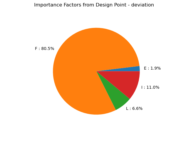
• the importance factors defined as the normalized director factors of the design point in the -space

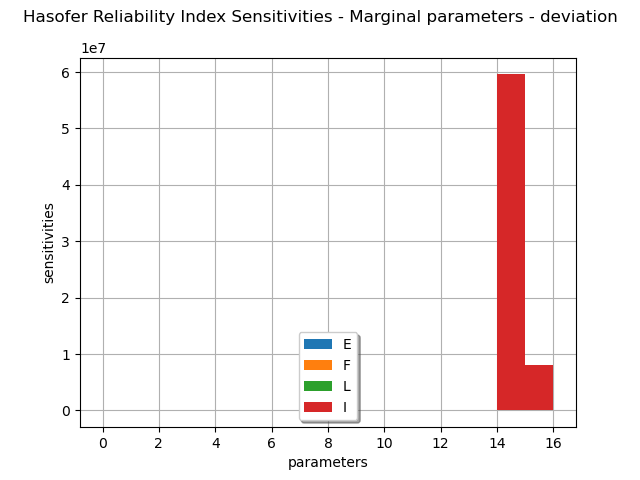
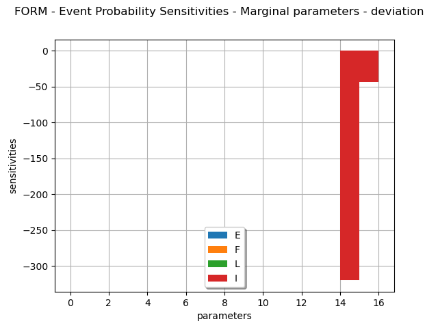
• the sensitivity factors of the Hasofer reliability index and the FORM probability,

• the coordinates of the mean point in the standard event space.

See FORM and SORM for theoretical details.

Model definition

from openturns.usecases import cantilever_beam
import openturns as ot
import openturns.viewer as viewer
from matplotlib import pylab as plt

ot.Log.Show(ot.Log.NONE)

We load the model from the usecases module :

cb = cantilever_beam.CantileverBeam()

We use the input parameters distribution from the data class :

distribution = cb.distribution
distribution.setDescription(["E", "F", "L", "I"])

We define the model

model = cb.model

Create the event whose probability we want to estimate.

vect = ot.RandomVector(distribution)
G = ot.CompositeRandomVector(model, vect)
event = ot.ThresholdEvent(G, ot.Greater(), 0.3)
event.setName("deviation")

FORM Analysis

Define a solver

optimAlgo = ot.Cobyla()
optimAlgo.setMaximumCallsNumber(1000)
optimAlgo.setMaximumAbsoluteError(1.0e-10)
optimAlgo.setMaximumRelativeError(1.0e-10)
optimAlgo.setMaximumResidualError(1.0e-10)
optimAlgo.setMaximumConstraintError(1.0e-10)

Run FORM

algo = ot.FORM(optimAlgo, event, distribution.getMean())
algo.run()
result = algo.getResult()

Analysis of the results

Probability

result.getEventProbability()

1.0900370418627377e-06

Hasofer reliability index

result.getHasoferReliabilityIndex()

4.735972259888528

Design point in the standard U* space.

print(result.getStandardSpaceDesignPoint())

[-0.665643,4.31264,1.23029,-1.3689]

Design point in the physical X space.

print(result.getPhysicalSpaceDesignPoint())

[6.56566e+10,458.976,2.58907,1.34803e-07]

Importance factors

graph = result.drawImportanceFactors()
view = viewer.View(graph)

marginalSensitivity, otherSensitivity = result.drawHasoferReliabilityIndexSensitivity()
marginalSensitivity.setLegends(["E", "F", "L", "I"])
marginalSensitivity.setLegendPosition("bottom")
view = viewer.View(marginalSensitivity)

marginalSensitivity, otherSensitivity = result.drawEventProbabilitySensitivity()
marginalSensitivity.setLegends(["E", "F", "L", "I"])
marginalSensitivity.setLegendPosition("bottom")
view = viewer.View(marginalSensitivity)

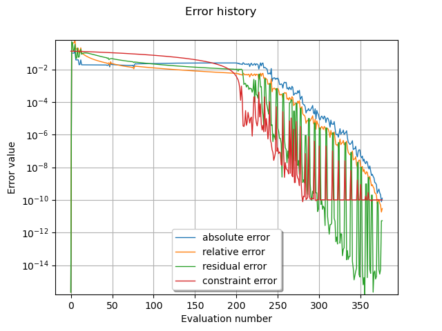
Error history

optimResult = result.getOptimizationResult()
graphErrors = optimResult.drawErrorHistory()
graphErrors.setLegendPosition("bottom")
graphErrors.setYMargin(0.0)
view = viewer.View(graphErrors)

Get additional results with SORM

algo = ot.SORM(optimAlgo, event, distribution.getMean())
algo.run()
sorm_result = algo.getResult()

Reliability index with Breitung approximation

sorm_result.getGeneralisedReliabilityIndexBreitung()

4.915018845541476

… with Hohenbichler approximation

sorm_result.getGeneralisedReliabilityIndexHohenbichler()

4.920394497861181

sorm_result.getGeneralisedReliabilityIndexTvedt()

4.923707817325712

SORM probability of the event with Breitung approximation

sorm_result.getEventProbabilityBreitung()

4.4386959812405013e-07

… with Hohenbichler approximation

sorm_result.getEventProbabilityHohenbichler()

4.318497365409196e-07

… with Tvedt approximation

sorm_result.getEventProbabilityTvedt()

plt.show()

FORM analysis with finite difference gradient

When the considered function has no analytical expression, the gradient may not be known. In this case, a constant step finite difference gradient definition may be used.

def cantilever_beam_python(X):
    E, F, L, II = X
    return [F * L**3 / (3 * E * II)]


cbPythonFunction = ot.PythonFunction(4, 1, func=cantilever_beam_python)
epsilon = [1e-8] * 4  # Here, a constant step of 1e-8 is used for every dimension
gradStep = ot.ConstantStep(epsilon)
cbPythonFunction.setGradient(
    ot.CenteredFiniteDifferenceGradient(gradStep, cbPythonFunction.getEvaluation())
)
G = ot.CompositeRandomVector(cbPythonFunction, vect)
event = ot.ThresholdEvent(G, ot.Greater(), 0.3)
event.setName("deviation")

However, given the different nature of the model variables, a blended (variable) finite difference step may be preferable: The step depends on the location in the input space

gradStep = ot.BlendedStep(epsilon)
cbPythonFunction.setGradient(
    ot.CenteredFiniteDifferenceGradient(gradStep, cbPythonFunction.getEvaluation())
)
G = ot.CompositeRandomVector(cbPythonFunction, vect)
event = ot.ThresholdEvent(G, ot.Greater(), 0.3)
event.setName("deviation")

We can then run the FORM analysis in the same way as before:

algo = ot.FORM(optimAlgo, event, distribution.getMean())
algo.run()
result = algo.getResult()