Estimate a process-based event probability¶

The objective of this example is to evaluate the probability of an event based on a stochastic process, using the Monte Carlo estimator.

Let $X: \Omega \times \mathcal{D} \rightarrow \mathbb{R}^d$ be a stochastic process of dimension $d$ , where $\mathcal{D} \in \mathbb{R}^n$ is discretized on the mesh $\mathcal{M}$ .

We define the event $\mathcal{E}$ as:

$\begin{aligned} \displaystyle \mathcal{E}(X) = \bigcup_{\underline{t}\in \mathcal{M}}\left\{X_{\underline{t}} \in \mathcal{A} \right\} \end{aligned}$

where $\mathcal{A}$ is a domain of $\mathbb{R}^d$ .

We estimate the probabilty $p=\mathbb{P}\left(\mathcal{E}(X)\right)$ with the Monte Carlo estimator.

The Monte Carlo algorithm is manipulated the same way as in the case where the event is based on a random variable independent of time.

We illustrate the algorithm on the example of the bidimensionnal white noise process $\varepsilon: \Omega \times \mathcal{D} \rightarrow \mathbb{R}^2$ where $\mathcal{D}\in \mathbb{R}$ , distributed according to the bidimensionnal standard normal distribution (with zero mean, unit variance and independent marginals).

We consider the domain $\mathcal{A} = [1,2] \times [1,2]$ . Then the event $\mathcal{E}$ writes:

$\begin{aligned} \displaystyle \mathcal{E}(\varepsilon) = \bigcup_{\underline{t}\in \mathcal{M}}\left\{\varepsilon_{t} \in \mathcal{A} \right\} \end{aligned}$

For all time stamps $t \in \mathcal{M}$ , the probability $p_1$ that the process enters into the domain $\mathcal{A}$ at time $t$ writes, using the independence property of the marginals:

$\begin{aligned} p_1 = \mathbb{P}\left(\varepsilon_t \in \mathcal{A}\right) = (\Phi(2) - \Phi(1))^2 \end{aligned}$

with $\Phi$ the cumulative distribution function of the scalar standard Normal distribution.

As the process is discretized on a time grid of size $N$ and using the independence property of the white noise between two different time stamps and the fact that the white noise follows the same distribution at each time $t$ , the final probability $p$ writes:

$p = \mathbb{P}\left(\mathcal{E}(\varepsilon)\right) = 1 - (1 - p_1)^{N}$

With $K=10^4$ realizations, using the Monte Carlo estimator, we obtain $p_K = 0.1627$ , to be compared to the exact value $p=0.17008$ for a time grid of size $N=10$ .

import openturns as ot
import openturns.viewer as viewer
from matplotlib import pylab as plt

ot.Log.Show(ot.Log.NONE)

Create a time grid

tMin = 0.0
timeStep = 0.1
n = 100
tgrid = ot.RegularGrid(tMin, timeStep, n)

Create a normal process

amplitude = [5.0]
scale = [3.0]
model = ot.ExponentialModel(scale, amplitude)
process = ot.GaussianProcess(model, tgrid)

Create the 1-d domain A: [2.,5.]

lowerBound = [2.0]
upperBound = [5.0]
domain = ot.Interval(lowerBound, upperBound)

Create an event from a Process and a Domain

event = ot.ProcessEvent(process, domain)

Create the Monte-Carlo algorithm

montecarlo = ot.ProbabilitySimulationAlgorithm(event)

# Define the maximum number of simulations
montecarlo.setMaximumOuterSampling(1000)

# Define the block size
montecarlo.setBlockSize(100)

# Define the maximum coefficient of variation
montecarlo.setMaximumCoefficientOfVariation(0.0025)

# Run the algorithm
montecarlo.run()

# Get the result
montecarlo.getResult()

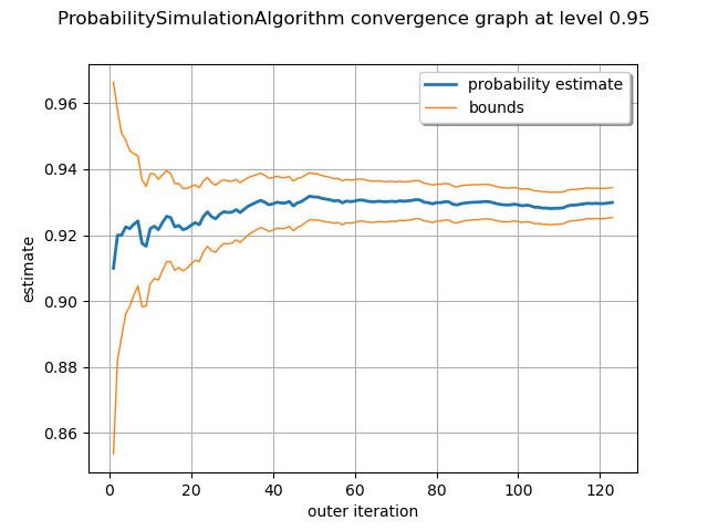
probabilityEstimate=9.299187e-01 varianceEstimate=5.351443e-06 standard deviation=2.31e-03 coefficient of variation=2.49e-03 confidenceLength(0.95)=9.07e-03 outerSampling=123 blockSize=100

graph = montecarlo.drawProbabilityConvergence(0.95)
view = viewer.View(graph)
plt.show()

ProbabilitySimulationAlgorithm convergence graph at level 0.95

OpenTURNS

An Open source initiative for the Treatment of Uncertainties, Risks'N Statistics

Previous topic

Next topic

This Page

Estimate a process-based event probability¶