AggregatedProcess¶

(Source code, png)

class AggregatedProcess(*args)¶

Aggregation of several processes in one process.

Parameters:

collProcsequence of Process: Collection of processes which all have the same input dimension.

Methods

`getClassName`()	Accessor to the object's name.
`getContinuousRealization`()	Get a continuous realization.
`getCovarianceModel`()	Accessor to the covariance model.
`getDescription`()	Get the description of the process.
`getFuture`(*args)	Prediction of the $N$ future iterations of the process.
`getInputDimension`()	Get the dimension of the domain $\cD$ .
`getMarginal`(*args)	Accessor the marginal processes.
`getMesh`()	Get the mesh.
`getName`()	Accessor to the object's name.
`getOutputDimension`()	Get the dimension of the domain $\cD$ .
`getProcessCollection`()	Get the collection of processes.
`getRealization`()	Get one realization of the aggregated process.
`getSample`(size)	Get $n$ realizations of the process.
`getTimeGrid`()	Get the time grid of observation of the process.
`getTrend`()	Accessor to the trend.
`hasName`()	Test if the object is named.
`isComposite`()	Test whether the process is composite or not.
`isNormal`()	Test whether the process is normal or not.
`isStationary`()	Test whether the process is stationary or not.
`setDescription`(description)	Set the description of the process.
`setMesh`(mesh)	Set the mesh.
`setName`(name)	Accessor to the object's name.
`setProcessCollection`(coll)	Set the collection of processes.
`setTimeGrid`(timeGrid)	Set the time grid of observation of the process.

Notes

If we note $X_i: \Omega \times\cD_i \mapsto \Rset^{d_i}$ for $0 \leq i \leq N$ the collection of processes, where $\cD_i \in \Rset^n$ for all $i$ . Then the resulting aggregated process $Y: \Omega \times\cD_0 \mapsto \Rset^d$ where $d=\sum_{i=0}^N d_i$ . The mesh of the first process $X_0$ has been assigned to the process $Y$ .

Examples

Create an aggregated process:

>>> import openturns as ot
>>> myMesher = ot.IntervalMesher([5, 10])
>>> lowerbound = [0.0, 0.0]
>>> upperBound = [2.0, 4.0]
>>> myInterval = ot.Interval(lowerbound, upperBound)
>>> myMesh = myMesher.build(myInterval)
>>> myProcess1 = ot.WhiteNoise(ot.Normal(), myMesh)
>>> myProcess2 = ot.WhiteNoise(ot.Triangular(), myMesh)
>>> myAggregatedProcess = ot.AggregatedProcess([myProcess1, myProcess2])

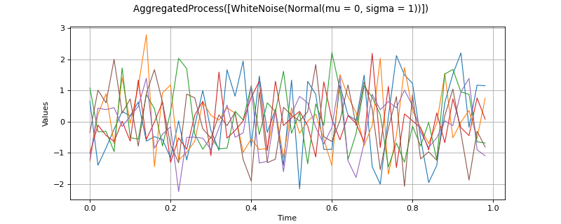
Draw one realization:

>>> myGraph = myAggregatedProcess.getRealization().drawMarginal(0)

__init__(*args)¶

getClassName()¶

Accessor to the object’s name.

Returns:

class_namestr: The object class name (object.__class__.__name__).

getContinuousRealization()¶

Get a continuous realization.

Returns:

realizationFunction: Each process of the collection is continuously realized on the common domain $\cD_0$ .

getCovarianceModel()¶

Accessor to the covariance model.

Returns:

cov_modelCovarianceModel: Covariance model, if any.

getDescription()¶

Get the description of the process.

Returns:

descriptionDescription: Description of the process.

getFuture(*args)¶

Prediction of the $N$ future iterations of the process.

Parameters:

stepNumberint, $N \geq 0$: Number of future steps.
sizeint, $size \geq 0$ , optional: Number of futures needed. Default is 1.

Returns:

predictionProcessSample or TimeSeries: $N$ future iterations of the process. If $size = 1$ , prediction is a TimeSeries. Otherwise, it is a ProcessSample.

getInputDimension()¶

Get the dimension of the domain $\cD$ .

Returns:

nint: Dimension of the domain $\cD$ : $n$ .

getMarginal(*args)¶

Accessor the marginal processes.

Available usages:

getMarginal(index)

getMarginal(indices)

Parameters:

indexint: Index of the selected marginal process.
indicesIndices: List of indices of the selected marginal processes.

Notes

The selected marginal processes are extracted if the list of indices does not mingle the processes of the initial collection: take care to extract all the marginal processes process by process. For example, if $X_0=(X_0^0, X_0^1)$ , $X_1=(X_1^0, X_1^1)$ and $X_2=(X_2^0, X_2^1, X_2^2)$ then you can extract Indices([1,0,2,4,6]) but not Indices([1,2,0,4,6]).

getMesh()¶

Get the mesh.

Returns:

meshMesh: Mesh over which the domain $\cD$ is discretized.

getName()¶

Accessor to the object’s name.

Returns:

namestr: The name of the object.

getOutputDimension()¶

Get the dimension of the domain $\cD$ .

Returns:

dint: Dimension of the domain $\cD$ .

getProcessCollection()¶

Get the collection of processes.

Returns:

collProcProcessCollection: Collection of processes which all have the same input dimension.

getRealization()¶

Get one realization of the aggregated process.

Returns:

realizationField: Each process of the collection is realized on the common mesh defined on $\cD_0$ .

getSample(size)¶

Get $n$ realizations of the process.

Parameters:

nint, $n \geq 0$: Number of realizations of the process needed.

Returns:

processSampleProcessSample: $n$ realizations of the random process. A process sample is a collection of fields which share the same mesh $\cM \in \Rset^n$ .

getTimeGrid()¶

Get the time grid of observation of the process.

Returns:

timeGridRegularGrid: Time grid of a process when the mesh associated to the process can be interpreted as a RegularGrid. We check if the vertices of the mesh are scalar and are regularly spaced in $\Rset$ but we don’t check if the connectivity of the mesh is conform to the one of a regular grid (without any hole and composed of ordered instants).

getTrend()¶

Accessor to the trend.

Returns:

trendTrendTransform: Trend, if any.

hasName()¶

Test if the object is named.

Returns:

hasNamebool: True if the name is not empty.

isComposite()¶

Test whether the process is composite or not.

Returns:

isCompositebool: True if the process is composite (built upon a function and a process).

isNormal()¶

Test whether the process is normal or not.

Returns:

isNormalbool: True if the process is normal.

Notes

A stochastic process is normal if all its finite dimensional joint distributions are normal, which means that for all $k \in \Nset$ and $I_k \in \Nset^*$ , with $cardI_k=k$ , there is $\vect{m}_1, \dots, \vect{m}_k \in \Rset^d$ and $\mat{C}_{1,\dots,k}\in\mathcal{M}_{kd,kd}(\Rset)$ such that:

$\Expect{\exp\left\{i\Tr{\vect{X}}_{I_k} \vect{U}_{k} \right\}} = \exp{\left\{i\Tr{\vect{U}}_{k}\vect{M}_{k}-\frac{1}{2}\Tr{\vect{U}}_{k}\mat{C}_{1,\dots,k}\vect{U}_{k}\right\}}$

where $\Tr{\vect{X}}_{I_k} = (\Tr{X}_{\vect{t}_1}, \hdots, \Tr{X}_{\vect{t}_k})$ , $\\Tr{vect{U}}_{k} = (\Tr{\vect{u}}_{1}, \hdots, \Tr{\vect{u}}_{k})$ and $\Tr{\vect{M}}_{k} = (\Tr{\vect{m}}_{1}, \hdots, \Tr{\vect{m}}_{k})$ and $\mat{C}_{1,\dots,k}$ is the symmetric matrix:

$\mat{C}_{1,\dots,k} = \left( \begin{array}{cccc} C(\vect{t}_1, \vect{t}_1) &C(\vect{t}_1, \vect{t}_2) & \hdots & C(\vect{t}_1, \vect{t}_{k}) \\ \hdots & C(\vect{t}_2, \vect{t}_2) & \hdots & C(\vect{t}_2, \vect{t}_{k}) \\ \hdots & \hdots & \hdots & \hdots \\ \hdots & \hdots & \hdots & C(\vect{t}_{k}, \vect{t}_{k}) \end{array} \right)$

A Gaussian process is entirely defined by its mean function $m$ and its covariance function $C$ (or correlation function $R$ ).

isStationary()¶

Test whether the process is stationary or not.

Returns:

isStationarybool: True if the process is stationary.

Notes

A process $X$ is stationary if its distribution is invariant by translation: $\forall k \in \Nset$ , $\forall (\vect{t}_1, \dots, \vect{t}_k) \in \cD$ , $\forall \vect{h}\in \Rset^n$ , we have:

$(X_{\vect{t}_1}, \dots, X_{\vect{t}_k}) \stackrel{\mathcal{D}}{=} (X_{\vect{t}_1+\vect{h}}, \dots, X_{\vect{t}_k+\vect{h}})$

setDescription(description)¶

Set the description of the process.

Parameters:

descriptionsequence of str: Description of the process.

setMesh(mesh)¶

Set the mesh.

Parameters:

meshMesh: Mesh over which the domain $\cD$ is discretized.

setName(name)¶

Accessor to the object’s name.

Parameters:

namestr: The name of the object.

setProcessCollection(coll)¶

Set the collection of processes.

Parameters:

collProcsequence of Process: Collection of processes which all have the same input dimension.

setTimeGrid(timeGrid)¶

Set the time grid of observation of the process.

Returns:

timeGridRegularGrid: Time grid of observation of the process when the mesh associated to the process can be interpreted as a RegularGrid. We check if the vertices of the mesh are scalar and are regularly spaced in $\Rset$ but we don’t check if the connectivity of the mesh is conform to the one of a regular grid (without any hole and composed of ordered instants).