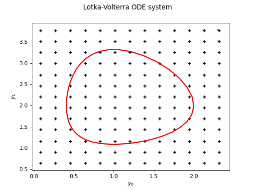
Fehlberg¶

(Source code, png)

class Fehlberg(*args)¶

Adaptive order Fehlberg method.

Parameters:

transitionFunctionFunction: The function defining the flow of the ordinary differential equation. Must have one parameter.
localPrecisionfloat: The expected absolute error on one step.
orderint, $order\in\{0,1,2,3,4\}$: The order of the method, ie the exponent $p$ in the estimate of the local error for a step of size $h$ written as $\cO(h^p)$ .

Methods

`getClassName`()	Accessor to the object's name.
`getName`()	Accessor to the object's name.
`getTransitionFunction`()	Transition function accessor.
`hasName`()	Test if the object is named.
`setName`(name)	Accessor to the object's name.
`setTransitionFunction`(transitionFunction)	Transition function accessor.
`solve`(*args)	Solve ODE.

See also

ODESolver

Notes

The Fehlberg method of order $p\in\Nset$ is a one-step explicit method made of two embedded Runge Kutta methods of order $p$ and $p+1$ . More precisely, such a method approximate the solution of:

$\vect{y}'(t)=f\left(t,\vect{y}(t)\right)\quad\mbox{with}\quad \vect{y}(t_0)=\vect{y}_0$

at a given set of locations $t_0,\dots,t_N$ by first building an approximation over an adapted grid $\tau_0=t_0,\dots,\tau_M=t_N$ with a number of points $M$ not necessarily equal to the number of locations $N$ and internal nodes not necessarily part of the set of locations. Then, the solution $\vect{y}$ is approximated by a smooth piecewise polynomial function using PiecewiseHermiteEvaluation, which is evaluated over the set of locations.

The method proceeds as follows. Knowing the solution at location $\vect{y}_i=\vect{y}(\tau_i)$ and a current time step $h_i$ , two approximations $\hat{\vect{y}}_{i+1}$ and $\bar{\vect{y}}_{i+1}$ of $\vect{y}_{i+1}=\vect{y}(\tau_i+h_i)=\vect{y}(\tau_{i+1})$ are built, such that:

$\hat{\vect{y}}_{i+1}=\vect{y}_i+h_i\vect{\Phi}_{\mathrm{I}}\left(\tau_i, \vect{y}_i, h_i\right) \\ \bar{\vect{y}}_{i+1}=\vect{y}_i+h_i\vect{\Phi}_{\mathrm{II}}\left(\tau_i, \vect{y}_i, h_i\right)$

where we assume that:

$\left|\vect{\Phi}_{\mathrm{I}}\left(\tau_i,\vect{y}_i,h_i\right)-(\vect{y}_{i+1}-\vect{y}_i)/h_i\right|=\cO\left(h_i^p\right)\\ \left|\vect{\Phi}_{\mathrm{II}}\left(\tau_i, \vect{y}_i,h_i\right)-(\vect{y}_{i+1}-\vect{y}_i)/h_i\right|=\cO\left(h_i^{p+1}\right)$

The evolution operators $\vect{\Phi}_{\mathrm{I}}$ and $\vect{\Phi}_{\mathrm{II}}$ are constructed as follows:

$\vect{\Phi}_{\mathrm{I}}\left(\tau, \vect{y}_i, h_i\right)=\sum_{k=0}^p c_kf_k\left(\tau,\vect{y}_i; h_i\right)\\ \vect{\Phi}_{\mathrm{II}}\left(\tau, \vect{y}_i, h_i\right)=\sum_{k=0}^{p+1} \hat{c}_kf_k\left(\tau,\vect{y}_i; h_i\right)$

with $f_k=f_k\left(\tau,\vect{y}_i,h_i\right)=f\left(\tau+\alpha_kh_i,\vect{y}_i+h_i\sum_{\ell=0}^{k-1}\beta_{k\ell}f_{\ell}\right)$ . The most desirable property of these methods is their embedded nature: the high-order approximation reuses all the evaluations of $f$ needed by the low-order approximation. The coefficients $c_k$ , $\hat{c}_k$ , $\alpha_k$ and $\beta_{k\ell}$ fully specify the method.

For $p=0$ we have:

$k$	$\alpha_k$	$\beta_{k0}$	$c_k$	$\hat{c}_k$
0	0	0	1	1/2
1	1	1		1/2

For $p=1$ we have:

$k$	$\alpha_k$	$\beta_{k0}$	$\beta_{k1}$	$c_k$	$\hat{c}_k$
0	0	0		1/256	1/512
1	1/2	1/2		255/256	255/256
2	1	1/256	255/256		1/512

For $p=2$ we have:

$k$	$\alpha_k$	$\beta_{k0}$	$\beta_{k1}$	$\beta_{k2}$	$c_k$	$\hat{c}_k$
0	0	0			214/891	533/2106
1	1/4	1/4			1/33	0
2	27/40	-189/800	214/891		650/891	800/1053
3	1	729/800	1/35	650/891		-1/78

For $p>2$ the coefficients can be found eg in the C++ source code. For additional theory on these methods see [stoer1993], chapter 7.

Examples

>>> import openturns as ot
>>> f = ot.SymbolicFunction(['t', 'y0', 'y1'], ['t - y0', 'y1 + t^2'])
>>> phi = ot.ParametricFunction(f, [0], [0.0])
>>> solver = ot.Fehlberg(phi)
>>> Y0 = [1.0, -1.0]
>>> nt = 100
>>> timeGrid = [(i**2.0) / (nt - 1.0)**2.0 for i in range(nt)]
>>> result = solver.solve(Y0, timeGrid)

__init__(*args)¶

getClassName()¶

Accessor to the object’s name.

Returns:

class_namestr: The object class name (object.__class__.__name__).

getName()¶

Accessor to the object’s name.

Returns:

namestr: The name of the object.

getTransitionFunction()¶

Transition function accessor.

Returns:

transitionFunctionFieldFunction: Transition function.

hasName()¶

Test if the object is named.

Returns:

hasNamebool: True if the name is not empty.

setName(name)¶

Accessor to the object’s name.

Parameters:

namestr: The name of the object.

setTransitionFunction(transitionFunction)¶

Transition function accessor.

Parameters:

transitionFunctionFieldFunction: Transition function.

solve(*args)¶

Solve ODE.

Parameters:

initialStatesequence of float: Initial value of the equation
timeGridsequence of float or Mesh of dimension 1: Time stamps, ie values of $t$ at which the solution is computed.

Returns:

valuesSample: The solution of the equation at grid points.

OpenTURNS

An Open source initiative for the Treatment of Uncertainties, Risks'N Statistics

Previous topic

Next topic

This Page

Fehlberg¶