Stiffened panel buckling¶

Introduction¶

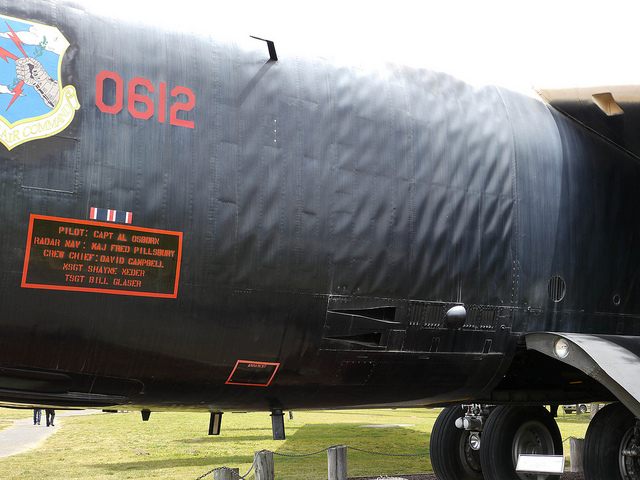
The following figure presents a stiffed panel subject to buckling on a military aircraft.

This use-case implements a simplified model of buckling for a stiffened panel (see [ko1994]).

buckling illustration — **Figure 1.** Buckling of a stiffened panel.¶

buckling simulation — **Figure 2.** 3D simulation of buckling.¶

stiffened panel geometry — **Figure 3.** Parameterization of the stiffened panel.¶

This test case is composed of ten random variables:

$E\sim\mathcal{TN}(\num{110.0e9}, \num{55.0e9}, \num{99.0e9}, \num{121.0e9})$ : Young modulus ( $\unit{\Pa}$ )
$nu\sim\mathcal{U}(0.3675, 0.3825)$ : Poisson coefficient (-)
$h_c\sim\mathcal{U}(0.0285, 0.0315)$ : Distance between the mean surface of the hat and the foot of the Stiffener ( $\unit{m}$ )
$\ell\sim\mathcal{U}(0.04655, 0.05145)$ : Length of the stiffener side ( $\unit{m}$ )
$f_1\sim\mathcal{U}(0.0266, 0.0294)$ : Width of the stiffener foot ( $\unit{m}$ )
$f_2\sim\mathcal{U}(0.00627, 0.00693)$ : Width of the stiffener hat ( $\unit{m}$ )
$t\sim\mathcal{U}(\num{8.02e-5}, \num{8.181e-5})$ : Thickness of the panel and the stiffener ( $\unit{m}$ )
$a\sim\mathcal{U}(0.6039, 0.6161)$ : Width of the panel ( $\unit{m}$ )
$b_0\sim\mathcal{U}(0.04455, 0.04545)$ : Distance between two stiffeners ( $\unit{m}$ )
$p\sim\mathcal{U}(0.03762, 0.03838)$ : Half-width of the stiffener ( $\unit{m}$ )

The output of interest is:

$(N_{xy})_{cr}$ : the critical shear force ( $\unit{N}$ )

We assume that the input variables are independent except the $f_1$ and $f_2$ for which we measure a Spearman correlation of $\rho^S_{12}=-0.8$ , modelled using a NormalCopula.

The critical load $(\tau_{xy})_{cr}$ of a stiffened panel subject to shear load is:

$(\tau_{xy})_{cr}=k_{xy}\frac{\pi^2D}{b_0^2t_s}$

where:

$a$ is the width of the panel;
$b_0$ is the width between too consecutive stiffener feet;
$t_s$ is the thickness of the panel main surface;
$E_s$ is the Young modulus of the panel main surface;
$\nu_s$ is the Poisson coefficient of the panel main surface;
$D$ is the bending coefficient of the panel main surface:

$k_{xy}$ is the load factor associated to shear buckling. It is given as a function of $\frac{b_0}{a}$ through the empirical equation:

$k_{xy} = 5.35 + 4 \left(\frac{b_0}{a}\right)^2.$

It is more convenient to use the shear force $N_{xy}$ instead of the shear stress component $\tau_{xy}$ . It leads to the equation:

$N_{xy}=q_1+q_c$

where $q_1$ abd $q_c$ are the shear fluxes in the panel main surface and its stiffener. They are given by:

$q_1=\tau_{xy}t_s=2G_sh_0t_s\frac{\partial^2w}{\partial x\partial y}$

and:

$q_c=\frac{G_ct_cp}{\ell} \left(h - 2h_0 + \frac{h_c}{2p}(f_1-f_2)\right) \frac{\partial^2w}{\partial x\partial y}$

where:

$G_s$ is the shear modulus of the panel main surface:

$G_s = \frac{E_s}{2(1 + \nu_s)};$

$\frac{\partial^2w}{\partial x\partial y}$ is the torsion strain of the panel main surface;
$G_c$ is the shear coefficient of the stiffener:

$G_c = \frac{E_c}{2(1 + \nu_c)};$

$t_c$ is the thickness of the stiffener;
$h_c$ is the distance between the mean surfaces of the stiffener hat and foot;
$h$ is the distance between the mean surfaces of the stiffener hat and the panel main surface:

$h = h_c+\frac{t_c + t_s}{2};$

$f_1$ is the width of the foot of the stiffener;
$f_2$ is the width of the hat of the stiffener;
$p$ is the half-widht of the stiffener;
$R$ is the radius of the circular part of the stiffener;
$\theta$ is the angle of the circular part of the stiffener;
$\ell$ is the length of the stiffener flank;
$d=\frac{\ell-f_2}{2}-R\theta$ is the half-lenght of the straight part of the side of the stiffener;
$A=\ell t_c$ is the area of the section of an half-ondulation;
$\bar{A}$ is the area of the section of the full panel (main surface and stiffener) bounded by $p$ :

$\bar{A} = A + pt_s + \frac{1}{2}(f_1 - f_2)t_c$

$h_0$ is the distance between the mean surface of the panel main surface and the global geometric center of the panel:

$h_0 = \frac{1}{2\bar{A}} \left(A(h_c+t_c+t_s)+\frac{1}{2}t_c(f_1-f_2)(t_c+t_s)\right).$

It leads to:

$N_{xy}=q_1(1+q_c/q_1) = \tau_{xy}t_s \left(1 + \frac{1}{4}\frac{G_ct_c}{G_st_s} \frac{2p(h-2h_0) - h_c(f_1-f_2)}{h_0\ell}\right)$

and finally, $(N_{xy})_{cr}$ is given by:

$(N_{xy})_{cr}=\left(5.35 + 4\left(\frac{b_0}{a}\right)^2\right)\left(\frac{\pi^2}{b_0^2}\frac{E_st_s^3}{12(1-\nu_s^2)}\right)\left(1+\frac{1}{4}\frac{G_ct_c}{G_st_s}\frac{2p(h-2h_0)-h_c(f_1-f_2)}{h_0\ell}\right)$

For industrial constraints, the stiffener and the main surface are cut in the same metal sheet, so $E_c=E_s=E$ , $\nu_c=\nu_s=\nu$ , $t_c=t_s=t$ . The final expression of the critical shear force is then:

$(N_{xy})_{cr}=\left(5.35 + 4\left(\frac{b_0}{a}\right)^2\right)\left(\frac{\pi^2}{b_0^2}\frac{Et^3}{12(1-\nu^2)}\right)\left(1+\frac{1}{4}\frac{2p(h-2h_0)-h_c(f_1-f_2)}{h_0\ell}\right)$

with:

$A=\ell t$ ;
$\bar{A}=A+t\left(p+\frac{f_1-f_2}{2}\right)$ ;
$h_0=\frac{A(h_c+2t)+t^2(f_1-f_2)}{2\bar{A}}$ ;
$h=h_c+t$ .

References¶

[ko1994]

Load the use case¶

We can load this model from the use cases module as follows :

>>> from openturns.usecases import stiffened_panel
>>> sp = stiffened_panel.StiffenedPanel()
>>> # Load the stiffened panel use case
>>> model = sp.model()

API documentation¶

class StiffenedPanel

Data class for the stiffened panel model.

Attributes:

dimint: The dimension of the problem, dim=10
modelSymbolicFunction: Model of the critical shearing load. The model has input dimension 10 and output dimension 1. More precisely, we have $\vect{X} = (E, \nu, h_c, \ell, f_1, f_2, t, a, b_0, p)$ and $Y = (N_{xy})_{cr}$ .
ETruncatedNormal: Young modulus distribution (Pa), ot.TruncatedNormal(110.0e9, 55.0e9, 99.0e9, 121.0e9)
nuUniform: Poisson coefficient (-) distribution ot.Uniform(0.3675, 0.3825)
h_cUniform: Distance between the mean surface of the hat and the foot of the Stiffener (m) distribution ot.Uniform(0.0285, 0.0315)
ellUniform: Length of the stiffener flank (m) distribution ot.Uniform(0.04655, 0.05145)
f_1Uniform: Width of the stiffener foot (m) distribution ot.Uniform(0.0266, 0.0294)
f_2Uniform: Width of the stiffener hat (m) distribution ot.Uniform(0.00627, 0.00693)
tUniform: Thickness of the panel and the stiffener (m) distribution ot.Uniform(8.02e-5, 8.181e-5)
aUniform: Width of the panel (m) distribution ot.Uniform(0.6039, 0.6161)
b_0Uniform: Distance between two stiffeners (m) distribution ot.Uniform(0.04455, 0.04545)
pUniform: Half-width of the stiffener (m) distribution ot.Uniform(0.03762, 0.03838)
correlation_matrixCorrelationMatrix: The correlation matrix used for inputs dependence, mostly identity except for the term representing the interaction between variables $f_1$ and $f_2$ which is -0.8.
copulaNormalCopula: The (Normal) copula used to define the distribution of the input parameters.
distributionJointDistribution: The joint distribution of the input parameters.
independentDistributionJointDistribution: The joint distribution of the input parameters for the special case of independence.

Examples

>>> from openturns.usecases import stiffened_panel
>>> # Load the stiffened panel model
>>> panel = stiffened_panel.StiffenedPanel()
>>> print("Inputs:", panel.model.getInputDescription())
Inputs: [E,nu,h_c,ell,f_1,f_2,t,a,b_0,p]
>>> print("Outputs:", panel.model.getOutputDescription())
Outputs: [(N_{xy})_{cr}]

Examples based on this use case¶

Estimate a buckling probability

OpenTURNS

An Open source initiative for the Treatment of Uncertainties, Risks'N Statistics

Table of Contents

Previous topic

Next topic

This Page