Note
Go to the end to download the full example code.
Calibration of the deflection of a tube
In this example, we calibrate the deflection of a tube as described in the use cases section. More precisely, we calibrate the mechanical parameters of a physical model which computes the vertical deflection of a tube and two deflection angles. This example shows how to calibrate a computer code which has several outputs.
In this example, we use Gaussian calibration method to calibrate the parametric model. Please read Gaussian calibration for more details on Bayesian Gaussian calibration. This study is relatively complicated: please read the calibration of the Chaboche mechanical model first if this is not already done.
Variables
In this this model, the following list presents which variables are observed input variables, input calibrated parameters and observed output variables.
F, E: Input. Observed.
L, a, D, d: Input. Calibrated.
 ,
,  ,
,  : Output. Observed.
from openturns.usecases import deflection_tube
import openturns as ot
import openturns.viewer as otv
from matplotlib import pylab as plt

ot.Log.Show(ot.Log.NONE)
Create a calibration problem
We load the model from the use case module :
dt = deflection_tube.DeflectionTube()
print("Inputs:", dt.model.getInputDescription())
print("Outputs:", dt.model.getOutputDescription())
Inputs: [F,L,a,De,di,E]
Outputs: [Deflection,Left angle,Right angle]
We see that there are 6 inputs: F, L, a, De, di, E and 3 outputs: Deflection, Left angle, Right angle. In this calibration example, the variables F and E are observed inputs and the input parameters L, a, De, di are calibrated.
We create a sample out of our input distribution :
sampleSize = 100
inputSample = dt.inputDistribution.getSample(sampleSize)
inputSample[0:5]
We take the image of our input sample by the model :
outputDeflection = dt.model(inputSample)
outputDeflection[0:5]
We now define the observed noise of the output. Since there are three observed outputs, there are three different standard deviations to define. Then we define a 3x3 covariance matrix of the observed outputs.
observationNoiseSigma = [0.1e-6, 0.5e-6, 0.5e-6]
observationNoiseCovariance = ot.CovarianceMatrix(3)
for i in range(3):
    observationNoiseCovariance[i, i] = observationNoiseSigma[i] ** 2
Finally, we define a dimension 3 normal distribution of the observed output and get a sample from it. We add this noise to the output of the model, which defines the observed output.
noiseSigma = ot.Normal([0.0, 0.0, 0.0], observationNoiseCovariance)
sampleObservationNoise = noiseSigma.getSample(sampleSize)
observedOutput = outputDeflection + sampleObservationNoise
observedOutput[0:5]
We now extract the observed inputs from the input sample.
observedInput = ot.Sample(sampleSize, 2)
observedInput[:, 0] = inputSample[:, 0]  # F
observedInput[:, 1] = inputSample[:, 5]  # E
observedInput.setDescription(["Force", "Young Modulus"])
observedInput[0:5]
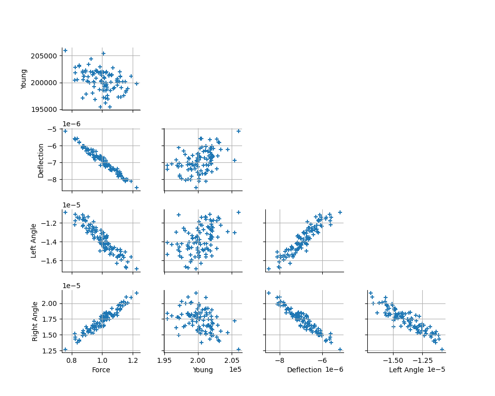
We would like to see how the observed output depend on the
observed inputs.
To do this, we use the DrawPairs() method.
fullSample = ot.Sample(sampleSize, 5)
fullSample[:, 0:2] = observedInput
fullSample[:, 2:5] = observedOutput
fullSample.setDescription(["Force", "Young", "Deflection", "Left Angle", "Right Angle"])
fullSample[0:5]
graph = ot.VisualTest.DrawPairs(fullSample)
view = otv.View(graph, figure_kw={"figsize": (10.0, 8.0)})
plt.subplots_adjust(wspace=0.3, hspace=0.3)
Setting up the calibration
Please consider that the input parameters L, a, De, di are calibrated. We define the initial point of the calibrated parameters: these values will be used as the mean of the prior normal distribution of the parameters. We set it with a slight difference with the true values, because, in general, we do not know the exact value (otherwise we would not use a calibration method).
XL = 1.4  # Exact : 1.5
Xa = 1.2  # Exact : 1.0
XD = 0.7  # Exact : 0.8
Xd = 0.2  # Exact : 0.1
thetaPrior = [XL, Xa, XD, Xd]
We now define the standard deviation of the prior distribution of the parameters. We compute the standard deviation as 10% of the value of the parameter. This ensures that the prior normal distribution has a spread which scales correctly with the mean of the Gaussian distribution. In other words, this setting corresponds to a 10% coefficient of variation.
sigmaXL = 0.1 * XL
sigmaXa = 0.1 * Xa
sigmaXD = 0.1 * XD
sigmaXd = 0.1 * Xd
parameterCovariance = ot.CovarianceMatrix(4)
parameterCovariance[0, 0] = sigmaXL**2
parameterCovariance[1, 1] = sigmaXa**2
parameterCovariance[2, 2] = sigmaXD**2
parameterCovariance[3, 3] = sigmaXd**2
print(parameterCovariance)
[[ 0.0196 0      0      0      ]
 [ 0      0.0144 0      0      ]
 [ 0      0      0.0049 0      ]
 [ 0      0      0      0.0004 ]]
In the physical model, the inputs and parameters are ordered as presented in the next table. Notice that there are no parameters in the physical model.
Index |
Input variable |
|---|---|
0 |
F |
1 |
L |
2 |
a |
3 |
De |
4 |
di |
5 |
E |
Index |
Parameter |
|---|---|
∅ |
∅ |
Table 1. Indices and names of the inputs and parameters of the physical model.
print("Physical Model Inputs:", dt.model.getInputDescription())
print("Physical Model Parameters:", dt.model.getParameterDescription())
Physical Model Inputs: [F,L,a,De,di,E]
Physical Model Parameters: []
In order to perform calibration, we have to define a parametric model,
with observed inputs and parameters to calibrate.
In order to do this, we create a ParametricFunction where the parameters
are L, a, de, di, which have the indices 1, 2, 3 and 4
in the physical model.
Index |
Input variable |
|---|---|
0 |
F |
1 |
E |
Index |
Parameter |
|---|---|
0 |
L |
1 |
a |
2 |
De |
3 |
di |
Table 2. Indices and names of the inputs and parameters of the parametric model.
calibratedIndices = [1, 2, 3, 4]  # [L, a, De, di]
calibrationFunction = ot.ParametricFunction(dt.model, calibratedIndices, thetaPrior)
print("Parametric Model Inputs:", calibrationFunction.getInputDescription())
print("Parametric Model Parameters:", calibrationFunction.getParameterDescription())
Parametric Model Inputs: [F,E]
Parametric Model Parameters: [L,a,De,di]
In the next cells, we are going to perform a Bayesian calibration,
based on Gaussian assumptions.
In the Bayesian framework, we define the standard deviation of the prior
Gaussian distribution of the observation errors.
Although the exact value of the standard deviation of the
observation errors is equal to 0.1e-6, we set slightly
different values because the value of the true standard deviation of
the observation error is not known in general.
We will be able to check if these hypotheses are correct
after calibration, using the drawResiduals() method.
sigmaObservation = [0.2e-6, 0.3e-6, 0.3e-6]  # Exact : [0.1e-6, 0.5e-6, 0.5e-6]
# Set the diagonal of the covariance matrix.
errorCovariance = ot.CovarianceMatrix(3)
errorCovariance[0, 0] = sigmaObservation[0] ** 2
errorCovariance[1, 1] = sigmaObservation[1] ** 2
errorCovariance[2, 2] = sigmaObservation[2] ** 2
calibrationFunction.setParameter(thetaPrior)
predictedOutput = calibrationFunction(observedInput)
predictedOutput[0:5]
Calibration with Gaussian non linear calibration
We are finally able to use the GaussianNonLinearCalibration.
algo = ot.GaussianNonLinearCalibration(
    calibrationFunction,
    observedInput,
    observedOutput,
    thetaPrior,
    parameterCovariance,
    errorCovariance,
)
The run() method launches the optimization algorithm.
algo.run()
calibrationResult = algo.getResult()
Analysis of the results
The getParameterMAP() method returns the optimized parameters.
thetaMAP = calibrationResult.getParameterMAP()
print("theta After = ", thetaMAP)
print("theta Before = ", thetaPrior)
theta After =  [1.50302,1.0039,0.801091,0.199872]
theta Before =  [1.4, 1.2, 0.7, 0.2]
Compute a 95% credibility interval for each marginal.
thetaPosterior = calibrationResult.getParameterPosterior()
alpha = 0.95
dim = thetaPosterior.getDimension()
for i in range(dim):
    print(thetaPosterior.getMarginal(i).computeBilateralConfidenceInterval(alpha))
[1.48179, 1.52491]
[0.978723, 1.02933]
[0.796699, 0.805538]
[0.199867, 0.199878]
We see that the parameters are accurately estimated in this case.
Increase the default number of points in the plots. This produces smoother spiky distributions.
ot.ResourceMap.SetAsUnsignedInteger("Distribution-DefaultPointNumber", 300)
In order to see how the predicted outputs first to the observed outputs, we plot the outputs depending on the inputs.
# sphinx_gallery_thumbnail_number = 2
graph = calibrationResult.drawObservationsVsInputs()
view = otv.View(
    graph,
    figure_kw={"figsize": (8.0, 6.0)},
    legend_kw={"bbox_to_anchor": (1.0, 1.0), "loc": "upper left"},
)
plt.subplots_adjust(wspace=0.3, hspace=0.7, right=0.8)
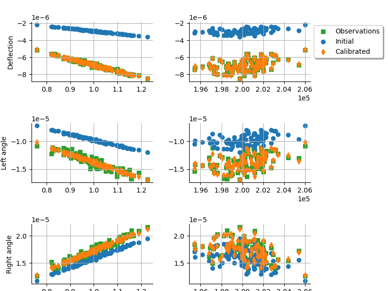
For all outputs, the predicted outputs of the model correspond to the observed outputs.
The next cell plots the predicted outputs depending on the observed outputs.
graph = calibrationResult.drawObservationsVsPredictions()
view = otv.View(
    graph,
    figure_kw={"figsize": (12.0, 4.0)},
    legend_kw={"bbox_to_anchor": (1.0, 1.0), "loc": "upper left"},
)
plt.subplots_adjust(wspace=0.3, left=0.05, right=0.85)
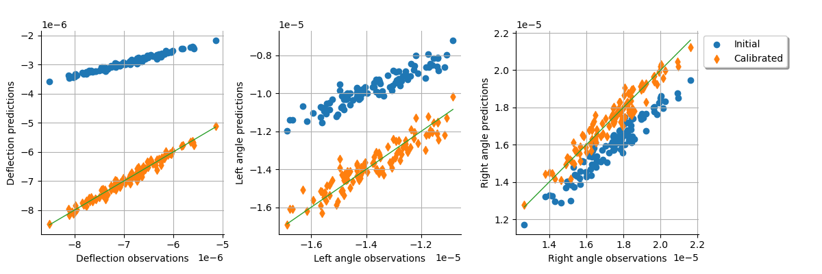
We see that, after calibration, the points are on the first diagonal of the plot: this shows that the calibration performs correctly.
In the next cell, we analyse the residuals before and after calibration. In order to clearly see these results, the next table presents the true standard deviation of the output error of observation compared to the hypothesis used in Gaussian calibration. In a practical study, the true sigma is unknown.
Output |
Sigma True |
Sigma hypothesis |
|---|---|---|
Deflection |
0.1e-6 |
0.2e-6 |
Left angle |
0.5e-6 |
0.3e-6 |
Right angle |
0.5e-6 |
0.3e-6 |
Table 3. For each output, the true standard deviation of the output error of observation compared to the hypothesis used in Gaussian calibration.
One of the hypotheses of the Gaussian calibration is that the observation errors are Gaussian. In order to check this hypothesis, we plot the distribution of the residuals before and after calibration. Furthermore, we plot the distribution of the observation errors, which is an hypothesis of the Gaussian calibration. Since there are three output, there are three residuals to check.
graph = calibrationResult.drawResiduals()
view = otv.View(
    graph,
    figure_kw={"figsize": (13.0, 4.0)},
    legend_kw={"bbox_to_anchor": (1.0, 1.0), "loc": "upper left"},
)
plt.subplots_adjust(wspace=0.3, left=0.05, right=0.7)
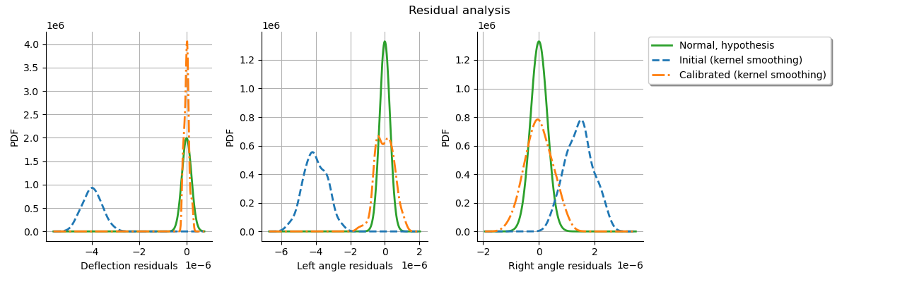
We see that the distribution of the residuals after calibration is centered on zero: this is a good point, since this shows that we have roughly equal chances to over or under predict the output when we use the calibrated model. We see that the distribution of each the residuals after calibration is relatively close to the Gaussian assumption that we used. For the first output, i.e. the deflection, the calibrated distribution of the residuals has a distribution which has spread lower than the hypothesis. This corresponds to the parameters that we used, since the true standard deviation of the errors is equal to 0.1e-6 while we used the 0.2e-6 hypothesis. The opposite happens for the left and right angle residuals: the calibrated residuals are narrower than the normal hypothesis that we used. This is because we used 0.3e-6 as the hypothesis while the true value is 0.05e-5.
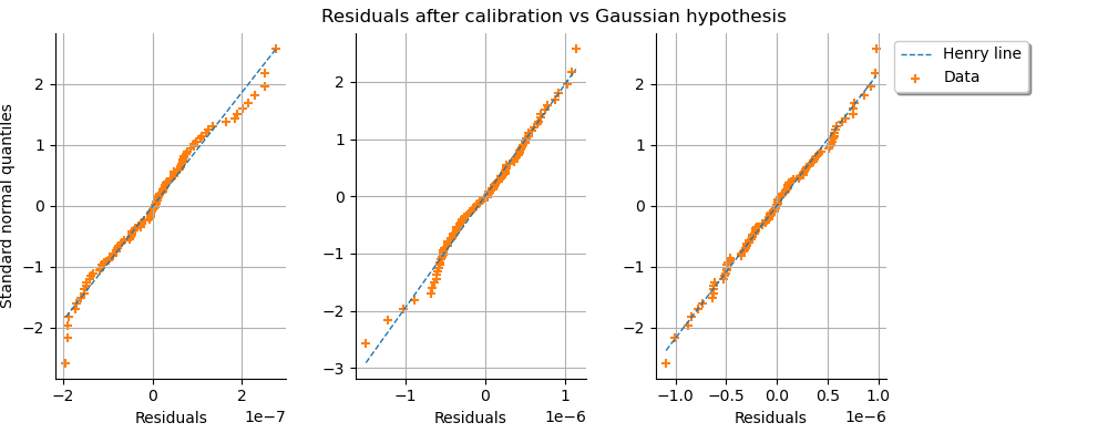
Check that the results are Gaussian, using a Normal-plot.
graph = calibrationResult.drawResidualsNormalPlot()
view = otv.View(
    graph,
    figure_kw={"figsize": (10.0, 4.0)},
    legend_kw={"bbox_to_anchor": (1.0, 1.0), "loc": "upper left"},
)
plt.subplots_adjust(wspace=0.3, left=0.05, right=0.8)
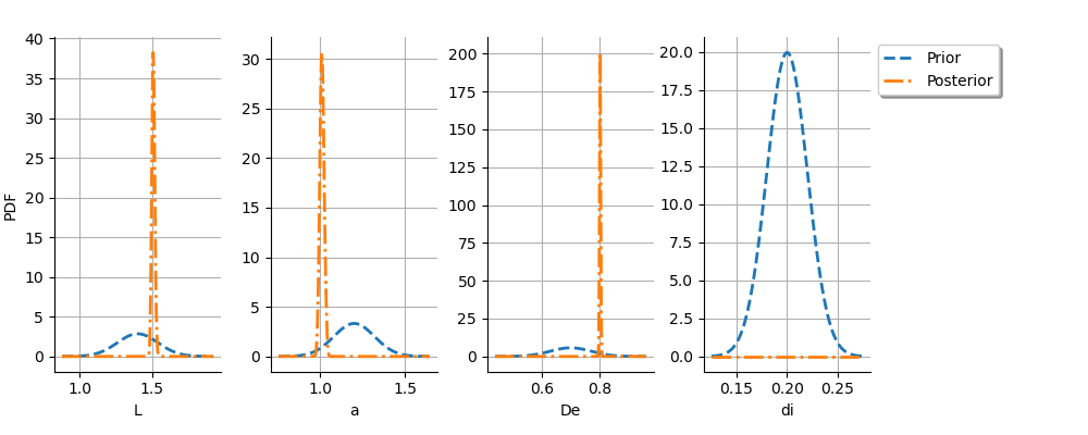
Finally, we observe the prior and posterior distribution of each parameter.
graph = calibrationResult.drawParameterDistributions()
view = otv.View(
    graph,
    figure_kw={"figsize": (10.0, 4.0)},
    legend_kw={"bbox_to_anchor": (1.0, 1.0), "loc": "upper left"},
)
plt.subplots_adjust(wspace=0.3, left=0.05, right=0.8)

otv.View.ShowAll()
Reset default settings
ot.ResourceMap.Reload()
Total running time of the script: (0 minutes 4.234 seconds)