Fit an extreme value distribution

import openturns as ot
import openturns.viewer as viewer
from matplotlib import pylab as plt

ot.Log.Show(ot.Log.NONE)

Set the random generator seed

ot.RandomGenerator.SetSeed(0)

The generalized extreme value distribution (GEV)

The GeneralizedExtremeValue distribution is a family of continuous probability distributions that combine the Gumbel, Frechet and WeibullMax distributions, all extreme value distributions.

In this example we use the associated GeneralizedExtremeValueFactory to fit sample with extreme values. This factory returns the best model among the Frechet, Gumbel and Weibull estimates according to the BIC criterion.

We draw a sample from a Gumbel of parameters and and another one from a Frechet with parameters , and . We consider both samples as a single sample from an unknown extreme distribution to be fitted.

The distributions used:

myGumbel = ot.Gumbel(1.0, 3.0)
myFrechet = ot.Frechet(1.0, 1.0, 0.0)

We build our experiment sample of size 2000.

sample = ot.Sample()
sampleFrechet = myFrechet.getSample(1000)
sampleGumbel = myGumbel.getSample(1000)
sample.add(sampleFrechet)
sample.add(sampleGumbel)

We fit the sample thanks to the GeneralizedExtremeValueFactory:

myDistribution = ot.GeneralizedExtremeValueFactory().buildAsGeneralizedExtremeValue(
    sample
)

We can display the parameters of the fitted distribution myDistribution:

print(myDistribution)

GeneralizedExtremeValue(mu=1.86805, sigma=1.58277, xi=0.454523)

We can also get the actual distribution (Weibull, Frechet or Gumbel) with the getActualDistribution method:

print(myDistribution.getActualDistribution())

Frechet(beta = 3.48225, alpha = 2.20011, gamma = -1.6142)

The given sample is then best described by a Frechet distribution.

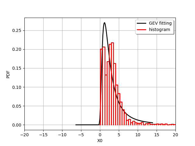
We draw the fitted distribution and a histogram of the data.

graph = myDistribution.drawPDF()
graph.add(ot.HistogramFactory().build(sample).drawPDF())
graph.setLegends(["GEV fitting", "histogram"])
graph.setLegendPosition("upper right")

view = viewer.View(graph)
axes = view.getAxes()
_ = axes[0].set_xlim(-20.0, 20.0)

We compare different fitting strategies for this sample:

• use the histogram from the data (red)

• the GEV fitted distribution (black)

• the pure Frechet fitted distribution (green)

• the pure Gumbel fitted distribution (blue)

• the pure WeibullMax fitted distribution (dashed orange)

graph = myDistribution.drawPDF()
graph.add(ot.HistogramFactory().build(sample).drawPDF())

distFrechet = ot.FrechetFactory().buildAsFrechet(sample)
graph.add(distFrechet.drawPDF())

distGumbel = ot.GumbelFactory().buildAsGumbel(sample)
graph.add(distGumbel.drawPDF())

# We change the line style of the WeibullMax.
distWeibullMax = ot.WeibullMaxFactory().buildAsWeibullMax(sample)
curveWeibullMax = distWeibullMax.drawPDF().getDrawable(0)
curveWeibullMax.setLineStyle("dashed")
graph.add(curveWeibullMax)

graph.setLegends(
    [
        "GEV fitting",
        "histogram",
        "Frechet fitting",
        "Gumbel fitting",
        "WeibullMax fitting",
    ]
)
graph.setLegendPosition("upper right")
view = viewer.View(graph)
axes = view.getAxes()  # axes is a matplotlib object
_ = axes[0].set_xlim(-20.0, 20.0)

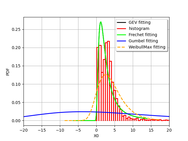
As returned by the getActualDistribution method the GEV distribution is a Frechet. The GeneralizedExtremeValueFactory class is a convenient class to fit extreme valued samples without an a priori knowledge of the underlying (at least the closest) extreme distribution.

The Generalized Pareto Distribution (GPD)

In this paragraph we fit a GeneralizedPareto distribution. Various estimators are provided by the GPD factory. Please refer to the GeneralizedParetoFactory class documentation for more information. The selection is based on the sample size and compared to the GeneralizedParetoFactory-SmallSize key of the ResourceMap:

print(ot.ResourceMap.GetAsUnsignedInteger("GeneralizedParetoFactory-SmallSize"))

20

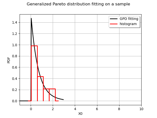
The small sample case

In this case the default estimator is based on a probability weighted method of moments, with a fallback on the exponential regression method.

myDist = ot.GeneralizedPareto(1.0, 0.0, 0.0)
N = 17
sample = myDist.getSample(N)

We build our experiment sample of size N.

myFittedDist = ot.GeneralizedParetoFactory().buildAsGeneralizedPareto(sample)
print(myFittedDist)

GeneralizedPareto(sigma = 0.678732, xi=0.0289962, u=0.0498077)

We draw the fitted distribution as well as an histogram to visualize the fit:

graph = myFittedDist.drawPDF()
graph.add(ot.HistogramFactory().build(sample).drawPDF())
graph.setTitle("Generalized Pareto distribution fitting on a sample")
graph.setLegends(["GPD fitting", "histogram"])
graph.setLegendPosition("upper right")

view = viewer.View(graph)
axes = view.getAxes()
_ = axes[0].set_xlim(-1.0, 10.0)

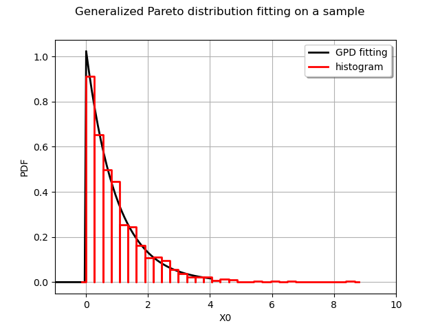
Large sample

For a larger sample the estimator is based on an exponential regression method with a fallback on the probability weighted moments estimator.

N = 1000
sample = myDist.getSample(N)

We build our experiment sample of size N.

myFittedDist = ot.GeneralizedParetoFactory().buildAsGeneralizedPareto(sample)
print(myFittedDist)

GeneralizedPareto(sigma = 0.971553, xi=-0.000639725, u=0.000103683)

We draw the fitted distribution as well as a histogram to visualize the fit:

graph = myFittedDist.drawPDF()
graph.add(ot.HistogramFactory().build(sample).drawPDF())
graph.setTitle("Generalized Pareto distribution fitting on a sample")
graph.setLegends(["GPD fitting", "histogram"])
graph.setLegendPosition("upper right")

view = viewer.View(graph)
axes = view.getAxes()
_ = axes[0].set_xlim(-1.0, 10.0)

plt.show()