Note
Go to the end to download the full example code.
Estimate a spectral density function
The objective of this example is to estimate the spectral density
function  from data, which can be a sample of time series or one time
series.
from data, which can be a sample of time series or one time
series.
The following example illustrates the case where the available data is a
sample of  realizations of the process, defined on the time grid
![[0, 102.3]](data:image/svg+xml;base64,PD94bWwgdmVyc2lvbj0nMS4wJyBlbmNvZGluZz0nVVRGLTgnPz4KPCEtLSBUaGlzIGZpbGUgd2FzIGdlbmVyYXRlZCBieSBkdmlzdmdtIDMuNC4yIC0tPgo8c3ZnIHZlcnNpb249JzEuMScgeG1sbnM9J2h0dHA6Ly93d3cudzMub3JnLzIwMDAvc3ZnJyB4bWxuczp4bGluaz0naHR0cDovL3d3dy53My5vcmcvMTk5OS94bGluaycgd2lkdGg9JzQ0LjI2NDA5NHB0JyBoZWlnaHQ9JzExLjk1NTE2OHB0JyB2aWV3Qm94PScwIC04Ljk2NjM3NiA0NC4yNjQwOTQgMTEuOTU1MTY4Jz4KPGRlZnM+CjxwYXRoIGlkPSdnMC01OCcgZD0nTTIuMTk5NzUxLS41NzM4NDhDMi4xOTk3NTEtLjkyMDU0OCAxLjkxMjgyNy0xLjE1OTY1MSAxLjYyNTkwMy0xLjE1OTY1MUMxLjI3OTIwMy0xLjE1OTY1MSAxLjA0MDEtLjg3MjcyNyAxLjA0MDEtLjU4NTgwM0MxLjA0MDEtLjIzOTEwMyAxLjMyNzAyNCAwIDEuNjEzOTQ4IDBDMS45NjA2NDggMCAyLjE5OTc1MS0uMjg2OTI0IDIuMTk5NzUxLS41NzM4NDhaJy8+CjxwYXRoIGlkPSdnMC01OScgZD0nTTIuMzMxMjU4IC4wNDc4MjFDMi4zMzEyNTgtLjY0NTU3OSAyLjEwNDExLTEuMTU5NjUxIDEuNjEzOTQ4LTEuMTU5NjUxQzEuMjMxMzgyLTEuMTU5NjUxIDEuMDQwMS0uODQ4ODE3IDEuMDQwMS0uNTg1ODAzUzEuMjE5NDI3IDAgMS42MjU5MDMgMEMxLjc4MTMyIDAgMS45MTI4MjctLjA0NzgyMSAyLjAyMDQyMy0uMTU1NDE3QzIuMDQ0MzM0LS4xNzkzMjggMi4wNTYyODktLjE3OTMyOCAyLjA2ODI0NC0uMTc5MzI4QzIuMDkyMTU0LS4xNzkzMjggMi4wOTIxNTQtLjAxMTk1NSAyLjA5MjE1NCAuMDQ3ODIxQzIuMDkyMTU0IC40NDIzNDEgMi4wMjA0MjMgMS4yMTk0MjcgMS4zMjcwMjQgMS45OTY1MTNDMS4xOTU1MTcgMi4xMzk5NzUgMS4xOTU1MTcgMi4xNjM4ODUgMS4xOTU1MTcgMi4xODc3OTZDMS4xOTU1MTcgMi4yNDc1NzIgMS4yNTUyOTMgMi4zMDczNDcgMS4zMTUwNjggMi4zMDczNDdDMS40MTA3MSAyLjMwNzM0NyAyLjMzMTI1OCAxLjQyMjY2NSAyLjMzMTI1OCAuMDQ3ODIxWicvPgo8cGF0aCBpZD0nZzEtNDgnIGQ9J001LjM1NTkxNS0zLjgyNTY1NEM1LjM1NTkxNS00LjgxNzkzMyA1LjI5NjEzOS01Ljc4NjMwMSA0Ljg2NTc1My02LjY5NDg5NEM0LjM3NTU5Mi03LjY4NzE3MyAzLjUxNDgxOS03Ljk1MDE4NyAyLjkyOTAxNi03Ljk1MDE4N0MyLjIzNTYxNi03Ljk1MDE4NyAxLjM4NjgtNy42MDM0ODcgLjk0NDQ1OC02LjYxMTIwOEMuNjA5NzE0LTUuODU4MDMyIC40OTAxNjItNS4xMTY4MTIgLjQ5MDE2Mi0zLjgyNTY1NEMuNDkwMTYyLTIuNjY2MDAyIC41NzM4NDgtMS43OTMyNzUgMS4wMDQyMzQtLjk0NDQ1OEMxLjQ3MDQ4Ni0uMDM1ODY2IDIuMjk1MzkyIC4yNTEwNTkgMi45MTcwNjEgLjI1MTA1OUMzLjk1NzE2MSAuMjUxMDU5IDQuNTU0OTE5LS4zNzA2MSA0LjkwMTYxOS0xLjA2NDAxQzUuMzMyMDA1LTEuOTYwNjQ4IDUuMzU1OTE1LTMuMTMyMjU0IDUuMzU1OTE1LTMuODI1NjU0Wk0yLjkxNzA2MSAuMDExOTU1QzIuNTM0NDk2IC4wMTE5NTUgMS43NTc0MS0uMjAzMjM4IDEuNTMwMjYyLTEuNTA2MzUxQzEuMzk4NzU1LTIuMjIzNjYxIDEuMzk4NzU1LTMuMTMyMjU0IDEuMzk4NzU1LTMuOTY5MTE2QzEuMzk4NzU1LTQuOTQ5NDQgMS4zOTg3NTUtNS44MzQxMjIgMS41OTAwMzctNi41Mzk0NzdDMS43OTMyNzUtNy4zNDA0NzMgMi40MDI5ODktNy43MTEwODMgMi45MTcwNjEtNy43MTEwODNDMy4zNzEzNTctNy43MTEwODMgNC4wNjQ3NTctNy40MzYxMTUgNC4yOTE5MDUtNi40MDc5N0M0LjQ0NzMyMy01LjcyNjUyNiA0LjQ0NzMyMy00Ljc4MjA2NyA0LjQ0NzMyMy0zLjk2OTExNkM0LjQ0NzMyMy0zLjE2ODEyIDQuNDQ3MzIzLTIuMjU5NTI3IDQuMzE1ODE2LTEuNTMwMjYyQzQuMDg4NjY3LS4yMTUxOTMgMy4zMzU0OTIgLjAxMTk1NSAyLjkxNzA2MSAuMDExOTU1WicvPgo8cGF0aCBpZD0nZzEtNDknIGQ9J00zLjQ0MzA4OC03LjY2MzI2M0MzLjQ0MzA4OC03LjkzODIzMiAzLjQ0MzA4OC03Ljk1MDE4NyAzLjIwMzk4NS03Ljk1MDE4N0MyLjkxNzA2MS03LjYyNzM5NyAyLjMxOTMwMy03LjE4NTA1NiAxLjA4NzkyLTcuMTg1MDU2Vi02LjgzODM1NkMxLjM2Mjg4OS02LjgzODM1NiAxLjk2MDY0OC02LjgzODM1NiAyLjYxODE4Mi03LjE0OTE5MVYtLjkyMDU0OEMyLjYxODE4Mi0uNDkwMTYyIDIuNTgyMzE2LS4zNDY3IDEuNTMwMjYyLS4zNDY3SDEuMTU5NjUxVjBDMS40ODI0NDEtLjAyMzkxIDIuNjQyMDkyLS4wMjM5MSAzLjAzNjYxMy0uMDIzOTFTNC41Nzg4MjktLjAyMzkxIDQuOTAxNjE5IDBWLS4zNDY3SDQuNTMxMDA5QzMuNDc4OTU0LS4zNDY3IDMuNDQzMDg4LS40OTAxNjIgMy40NDMwODgtLjkyMDU0OFYtNy42NjMyNjNaJy8+CjxwYXRoIGlkPSdnMS01MCcgZD0nTTUuMjYwMjc0LTIuMDA4NDY4SDQuOTk3MjZDNC45NjEzOTUtMS44MDUyMyA0Ljg2NTc1My0xLjE0NzY5NiA0Ljc0NjIwMi0uOTU2NDEzQzQuNjYyNTE2LS44NDg4MTcgMy45ODEwNzEtLjg0ODgxNyAzLjYyMjQxNi0uODQ4ODE3SDEuNDEwNzFDMS43MzM0OTktMS4xMjM3ODYgMi40NjI3NjUtMS44ODg5MTcgMi43NzM1OTktMi4xNzU4NDFDNC41OTA3ODUtMy44NDk1NjQgNS4yNjAyNzQtNC40NzEyMzMgNS4yNjAyNzQtNS42NTQ3OTVDNS4yNjAyNzQtNy4wMjk2MzkgNC4xNzIzNTQtNy45NTAxODcgMi43ODU1NTQtNy45NTAxODdTLjU4NTgwMy02Ljc2NjYyNSAuNTg1ODAzLTUuNzM4NDgxQy41ODU4MDMtNS4xMjg3NjcgMS4xMTE4MzEtNS4xMjg3NjcgMS4xNDc2OTYtNS4xMjg3NjdDMS4zOTg3NTUtNS4xMjg3NjcgMS43MDk1ODktNS4zMDgwOTUgMS43MDk1ODktNS42OTA2NkMxLjcwOTU4OS02LjAyNTQwNSAxLjQ4MjQ0MS02LjI1MjU1MyAxLjE0NzY5Ni02LjI1MjU1M0MxLjA0MDEtNi4yNTI1NTMgMS4wMTYxODktNi4yNTI1NTMgLjk4MDMyNC02LjI0MDU5OEMxLjIwNzQ3Mi03LjA1MzU0OSAxLjg1MzA1MS03LjYwMzQ4NyAyLjYzMDEzNy03LjYwMzQ4N0MzLjY0NjMyNi03LjYwMzQ4NyA0LjI2Nzk5NS02Ljc1NDY3IDQuMjY3OTk1LTUuNjU0Nzk1QzQuMjY3OTk1LTQuNjM4NjA1IDMuNjgyMTkyLTMuNzUzOTIzIDMuMDAwNzQ3LTIuOTg4NzkyTC41ODU4MDMtLjI4NjkyNFYwSDQuOTQ5NDRMNS4yNjAyNzQtMi4wMDg0NjhaJy8+CjxwYXRoIGlkPSdnMS01MScgZD0nTTIuMTk5NzUxLTQuMjkxOTA1QzEuOTk2NTEzLTQuMjc5OTUgMS45NDg2OTItNC4yNjc5OTUgMS45NDg2OTItNC4xNjAzOTlDMS45NDg2OTItNC4wNDA4NDcgMi4wMDg0NjgtNC4wNDA4NDcgMi4yMjM2NjEtNC4wNDA4NDdIMi43NzM1OTlDMy43ODk3ODgtNC4wNDA4NDcgNC4yNDQwODUtMy4yMDM5ODUgNC4yNDQwODUtMi4wNTYyODlDNC4yNDQwODUtLjQ5MDE2MiAzLjQzMTEzMy0uMDcxNzMxIDIuODQ1MzMtLjA3MTczMUMyLjI3MTQ4Mi0uMDcxNzMxIDEuMjkxMTU4LS4zNDY3IC45NDQ0NTgtMS4xMzU3NDFDMS4zMjcwMjQtMS4wNzU5NjUgMS42NzM3MjQtMS4yOTExNTggMS42NzM3MjQtMS43MjE1NDRDMS42NzM3MjQtMi4wNjgyNDQgMS40MjI2NjUtMi4zMDczNDcgMS4wODc5Mi0yLjMwNzM0N0MuODAwOTk2LTIuMzA3MzQ3IC40OTAxNjItMi4xMzk5NzUgLjQ5MDE2Mi0xLjY4NTY3OUMuNDkwMTYyLS42MjE2NjkgMS41NTQxNzIgLjI1MTA1OSAyLjg4MTE5NiAuMjUxMDU5QzQuMzAzODYxIC4yNTEwNTkgNS4zNTU5MTUtLjgzNjg2MiA1LjM1NTkxNS0yLjA0NDMzNEM1LjM1NTkxNS0zLjE0NDIwOSA0LjQ3MTIzMy00LjAwNDk4MSAzLjMyMzUzNy00LjIwODIxOUM0LjM2MzYzNi00LjUwNzA5OCA1LjAzMzEyNi01LjM3OTgyNiA1LjAzMzEyNi02LjMxMjMyOUM1LjAzMzEyNi03LjI1Njc4NyA0LjA1MjgwMi03Ljk1MDE4NyAyLjg5MzE1MS03Ljk1MDE4N0MxLjY5NzYzNC03Ljk1MDE4NyAuODEyOTUxLTcuMjIwOTIyIC44MTI5NTEtNi4zNDgxOTRDLjgxMjk1MS01Ljg2OTk4OCAxLjE4MzU2Mi01Ljc3NDM0NiAxLjM2Mjg4OS01Ljc3NDM0NkMxLjYxMzk0OC01Ljc3NDM0NiAxLjkwMDg3Mi01Ljk1MzY3NCAxLjkwMDg3Mi02LjMxMjMyOUMxLjkwMDg3Mi02LjY5NDg5NCAxLjYxMzk0OC02Ljg2MjI2NyAxLjM1MDkzNC02Ljg2MjI2N0MxLjI3OTIwMy02Ljg2MjI2NyAxLjI1NTI5My02Ljg2MjI2NyAxLjIxOTQyNy02Ljg1MDMxMUMxLjY3MzcyNC03LjY2MzI2MyAyLjc5NzUwOS03LjY2MzI2MyAyLjg1NzI4NS03LjY2MzI2M0MzLjI1MTgwNi03LjY2MzI2MyA0LjAyODg5Mi03LjQ4MzkzNSA0LjAyODg5Mi02LjMxMjMyOUM0LjAyODg5Mi02LjA4NTE4MSAzLjk5MzAyNi01LjQxNTY5MSAzLjY0NjMyNi00LjkwMTYxOUMzLjI4NzY3MS00LjM3NTU5MiAyLjg4MTE5Ni00LjMzOTcyNiAyLjU1ODQwNi00LjMyNzc3MUwyLjE5OTc1MS00LjI5MTkwNVonLz4KPHBhdGggaWQ9J2cxLTkxJyBkPSdNMi45ODg3OTIgMi45ODg3OTJWMi41NDY0NTFIMS44MjkxNDFWLTguNTI0MDM1SDIuOTg4NzkyVi04Ljk2NjM3NkgxLjM4NjhWMi45ODg3OTJIMi45ODg3OTJaJy8+CjxwYXRoIGlkPSdnMS05MycgZD0nTTEuODUzMDUxLTguOTY2Mzc2SC4yNTEwNTlWLTguNTI0MDM1SDEuNDEwNzFWMi41NDY0NTFILjI1MTA1OVYyLjk4ODc5MkgxLjg1MzA1MVYtOC45NjYzNzZaJy8+CjwvZGVmcz4KPGcgaWQ9J3BhZ2UxJz4KPHVzZSB4PScwJyB5PScwJyB4bGluazpocmVmPScjZzEtOTEnLz4KPHVzZSB4PSczLjI1MTY2MScgeT0nMCcgeGxpbms6aHJlZj0nI2cxLTQ4Jy8+Cjx1c2UgeD0nOS4xMDQ2NTInIHk9JzAnIHhsaW5rOmhyZWY9JyNnMC01OScvPgo8dXNlIHg9JzE0LjM0ODgxJyB5PScwJyB4bGluazpocmVmPScjZzEtNDknLz4KPHVzZSB4PScyMC4yMDE4MDEnIHk9JzAnIHhsaW5rOmhyZWY9JyNnMS00OCcvPgo8dXNlIHg9JzI2LjA1NDc5MScgeT0nMCcgeGxpbms6aHJlZj0nI2cxLTUwJy8+Cjx1c2UgeD0nMzEuOTA3NzgxJyB5PScwJyB4bGluazpocmVmPScjZzAtNTgnLz4KPHVzZSB4PSczNS4xNTk0NDInIHk9JzAnIHhsaW5rOmhyZWY9JyNnMS01MScvPgo8dXNlIHg9JzQxLjAxMjQzMycgeT0nMCcgeGxpbms6aHJlZj0nI2cxLTkzJy8+CjwvZz4KPC9zdmc+CjwhLS0gREVQVEg9NCAtLT4=) , discretized every
, discretized every  . The spectral model of
the process is the Cauchy model parameterized by
. The spectral model of
the process is the Cauchy model parameterized by  and
and  .
.
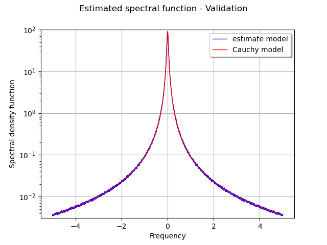
The figure draws the graph of the real spectral model and its estimation from the sample of time series.
import openturns as ot
import openturns.viewer as otv

ot.Log.Show(ot.Log.NONE)
Generate some data
# Create the time grid
# In the context of the spectral estimate or Fourier transform use,
# we use data blocs with size of form 2^p
tMin = 0.0
tstep = 0.1
size = 2**12
tgrid = ot.RegularGrid(tMin, tstep, size)

# We fix the parameter of the Cauchy model
amplitude = [5.0]
scale = [3.0]
model = ot.CauchyModel(amplitude, scale)
process = ot.SpectralGaussianProcess(model, tgrid)

# Get a time series or a sample of time series
tseries = process.getRealization()
sample = process.getSample(1000)
Build a spectral model factory
segmentNumber = 10
overlapSize = 0.3
factory = ot.WelchFactory(ot.Hann(), segmentNumber, overlapSize)
Estimation on a TimeSeries or on a ProcessSample
estimatedModel_TS = factory.build(tseries)
estimatedModel_PS = factory.build(sample)
Change the filtering window
factory.setFilteringWindows(ot.Hamming())
Get the frequencyGrid
frequencyGrid = ot.SpectralGaussianProcess(estimatedModel_PS, tgrid).getFrequencyGrid()
# With the model, we want to compare values
# We compare values computed with theoritical values
plotSample = ot.Sample(frequencyGrid.getN(), 3)

# Loop of comparison ==> data are saved in plotSample
for k in range(frequencyGrid.getN()):
    freq = frequencyGrid.getStart() + k * frequencyGrid.getStep()
    plotSample[k, 0] = freq
    plotSample[k, 1] = abs(estimatedModel_PS(freq)[0, 0])
    plotSample[k, 2] = abs(model(freq)[0, 0])

# Some cosmetics : labels, legend position, ...
graph = ot.Graph(
    "Estimated spectral function - Validation",
    "Frequency",
    "Spectral density function",
    True,
    "upper right",
)
graph.setLogScale(ot.GraphImplementation.LOGY)

# The first curve is the estimate density as function of frequency
curve1 = ot.Curve(plotSample.getMarginal([0, 1]))
curve1.setColor("blue")
curve1.setLegend("estimate model")

# The second curve is the theoritical density as function of frequency
curve2 = ot.Curve(plotSample.getMarginal([0, 2]))
curve2.setColor("red")
curve2.setLegend("Cauchy model")

graph.add(curve1)
graph.add(curve2)
view = otv.View(graph)
otv.View.ShowAll()