Kolmogorov-Smirnov : understand the statistics

In this example, we illustrate how the Kolmogorov-Smirnov (KS) statistic is computed.

• We generate a sample from a Normal distribution.

• We create a uniform distribution and estimate its parameters from the sample.

• Compute the Kolmogorov-Smirnov statistic and plot it on top of the empirical cumulated distribution function.

import openturns as ot
import openturns.viewer as viewer

ot.Log.Show(ot.Log.NONE)

The computeKSStatisticsIndex function computes the Kolmogorov-Smirnov distance between the sample and the distribution. Furthermore, it returns the index which achieves the maximum distance in the sorted sample. The following function is for teaching purposes only: use FittingTest for real applications.

def computeKSStatisticsIndex(sample, distribution):
    sample = ot.Sample(sample.sort())
    print("Sorted")
    print(sample)
    n = sample.getSize()
    D = 0.0
    index = -1
    D_previous = 0.0
    for i in range(n):
        F = distribution.computeCDF(sample[i])
        S1 = abs(F - float(i) / n)
        S2 = abs(float(i + 1) / n - F)
        print(
            "i=%d, x[i]=%.4f, F(x[i])=%.4f, S1=%.4f, S2=%.4f"
            % (i, sample[i, 0], F, S1, S2)
        )
        D = max(S1, S2, D)
        if D > D_previous:
            print("D max!")
            index = i
            D_previous = D
    observation = sample[index]
    return D, index, observation

The drawKSDistance() function plots the empirical distribution function of the sample and the Kolmogorov-Smirnov distance at point x. The empirical CDF is a staircase function and is discontinuous at each observation. Denote by the empirical CDF. For a given observation which achieves the maximum distance to the candidate distribution CDF, let us denote and . The maximum distance can be achieved either by or . The computeEmpiricalCDF(x) method computes . We compute with the equation where is the sample size.

def drawKSDistance(sample, distribution, observation, D, distFactory):
    graph = ot.Graph("KS Distance = %.4f" % (D), "X", "CDF", True, "upper left")
    # Thick vertical line at point x
    ECDF_x_plus = sample.computeEmpiricalCDF(observation)
    ECDF_x_minus = ECDF_x_plus - 1.0 / sample.getSize()
    CDF_index = distribution.computeCDF(observation)
    curve = ot.Curve(
        [observation[0], observation[0], observation[0]],
        [ECDF_x_plus, ECDF_x_minus, CDF_index],
    )
    curve.setLegend("KS Statistics")
    curve.setLineWidth(4.0 * curve.getLineWidth())
    graph.add(curve)
    # Empirical CDF
    empiricalCDF = ot.UserDefined(sample).drawCDF()
    empiricalCDF.setLegends(["Empirical DF"])
    graph.add(empiricalCDF)
    #
    distname = distFactory.getClassName()
    distribution = distFactory.build(sample)
    cdf = distribution.drawCDF()
    cdf.setLegends([distname])
    graph.add(cdf)
    return graph

We generate a sample from a standard Normal distribution.

N = ot.Normal()
n = 10
sample = N.getSample(n)

Compute the index which achieves the maximum Kolmogorov-Smirnov distance.

We then create a uniform distribution whose parameters are estimated from the sample. This way, the K.S. distance is large enough to be graphically significant.

distFactory = ot.UniformFactory()
distribution = distFactory.build(sample)
distribution

Uniform

• name=Uniform
• dimension=1
• weight=1
• range=[-2.13183, 0.941165]
• description=[X0]
• isParallel=true
• isCopula=false

Compute the index which achieves the maximum Kolmogorov-Smirnov distance.

D, index, observation = computeKSStatisticsIndex(sample, distribution)
print("D=", D, ", Index=", index, ", Obs.=", observation)

Sorted
0 : [ -1.91233   ]
1 : [ -1.66867   ]
2 : [ -1.27863   ]
3 : [ -1.02711   ]
4 : [ -0.67053   ]
5 : [ -0.320149  ]
6 : [ -0.0887425 ]
7 : [ -0.040941  ]
8 : [  0.506129  ]
9 : [  0.721665  ]
i=0, x[i]=-1.9123, F(x[i])=0.0714, S1=0.0714, S2=0.0286
D max!
i=1, x[i]=-1.6687, F(x[i])=0.1507, S1=0.0507, S2=0.0493
i=2, x[i]=-1.2786, F(x[i])=0.2776, S1=0.0776, S2=0.0224
D max!
i=3, x[i]=-1.0271, F(x[i])=0.3595, S1=0.0595, S2=0.0405
i=4, x[i]=-0.6705, F(x[i])=0.4755, S1=0.0755, S2=0.0245
i=5, x[i]=-0.3201, F(x[i])=0.5895, S1=0.0895, S2=0.0105
D max!
i=6, x[i]=-0.0887, F(x[i])=0.6649, S1=0.0649, S2=0.0351
i=7, x[i]=-0.0409, F(x[i])=0.6804, S1=0.0196, S2=0.1196
D max!
i=8, x[i]=0.5061, F(x[i])=0.8584, S1=0.0584, S2=0.0416
i=9, x[i]=0.7217, F(x[i])=0.9286, S1=0.0286, S2=0.0714
D= 0.1195927736833764 , Index= 7 , Obs.= [-0.040941]

graph = drawKSDistance(sample, distribution, observation, D, distFactory)
view = viewer.View(graph)

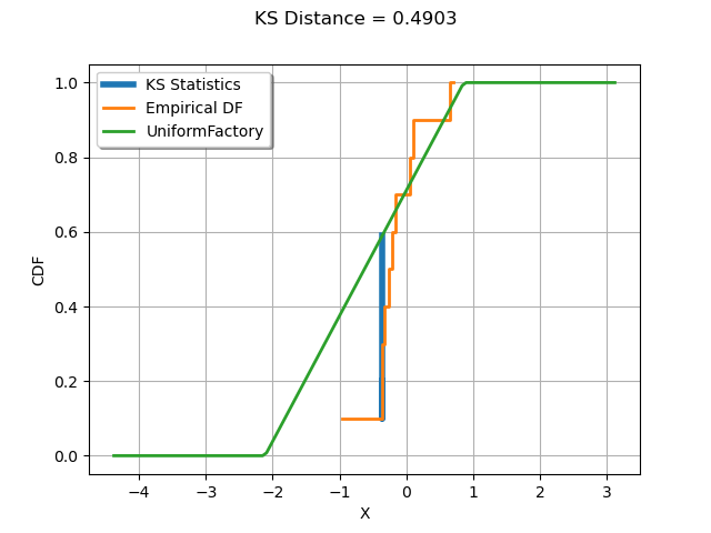
Display the graphs

view.ShowAll()

We see that the K.S. statistics is achieved at the observation where the distance between the empirical distribution function of the sample and the candidate distribution is largest.