Note
Go to the end to download the full example code.
Create a discrete Markov chain process
This example details first how to create and manipulate a discrete Markov chain.
A discrete Markov chain  , where
 ![E = [\![ 0,...,p-1]\!]](data:image/svg+xml;base64,PD94bWwgdmVyc2lvbj0nMS4wJyBlbmNvZGluZz0nVVRGLTgnPz4KPCEtLSBUaGlzIGZpbGUgd2FzIGdlbmVyYXRlZCBieSBkdmlzdmdtIDMuNC4yIC0tPgo8c3ZnIHZlcnNpb249JzEuMScgeG1sbnM9J2h0dHA6Ly93d3cudzMub3JnLzIwMDAvc3ZnJyB4bWxuczp4bGluaz0naHR0cDovL3d3dy53My5vcmcvMTk5OS94bGluaycgd2lkdGg9Jzg2LjU3MDQwM3B0JyBoZWlnaHQ9JzExLjk1NTE2OHB0JyB2aWV3Qm94PScwIC04Ljk2NjM3NiA4Ni41NzA0MDMgMTEuOTU1MTY4Jz4KPGRlZnM+CjxwYXRoIGlkPSdnMC0wJyBkPSdNNy44Nzg0NTYtMi43NDk2ODlDOC4wODE2OTQtMi43NDk2ODkgOC4yOTY4ODctMi43NDk2ODkgOC4yOTY4ODctMi45ODg3OTJTOC4wODE2OTQtMy4yMjc4OTUgNy44Nzg0NTYtMy4yMjc4OTVIMS40MTA3MUMxLjIwNzQ3Mi0zLjIyNzg5NSAuOTkyMjc5LTMuMjI3ODk1IC45OTIyNzktMi45ODg3OTJTMS4yMDc0NzItMi43NDk2ODkgMS40MTA3MS0yLjc0OTY4OUg3Ljg3ODQ1NlonLz4KPHBhdGggaWQ9J2cyLTQ4JyBkPSdNNS4zNTU5MTUtMy44MjU2NTRDNS4zNTU5MTUtNC44MTc5MzMgNS4yOTYxMzktNS43ODYzMDEgNC44NjU3NTMtNi42OTQ4OTRDNC4zNzU1OTItNy42ODcxNzMgMy41MTQ4MTktNy45NTAxODcgMi45MjkwMTYtNy45NTAxODdDMi4yMzU2MTYtNy45NTAxODcgMS4zODY4LTcuNjAzNDg3IC45NDQ0NTgtNi42MTEyMDhDLjYwOTcxNC01Ljg1ODAzMiAuNDkwMTYyLTUuMTE2ODEyIC40OTAxNjItMy44MjU2NTRDLjQ5MDE2Mi0yLjY2NjAwMiAuNTczODQ4LTEuNzkzMjc1IDEuMDA0MjM0LS45NDQ0NThDMS40NzA0ODYtLjAzNTg2NiAyLjI5NTM5MiAuMjUxMDU5IDIuOTE3MDYxIC4yNTEwNTlDMy45NTcxNjEgLjI1MTA1OSA0LjU1NDkxOS0uMzcwNjEgNC45MDE2MTktMS4wNjQwMUM1LjMzMjAwNS0xLjk2MDY0OCA1LjM1NTkxNS0zLjEzMjI1NCA1LjM1NTkxNS0zLjgyNTY1NFpNMi45MTcwNjEgLjAxMTk1NUMyLjUzNDQ5NiAuMDExOTU1IDEuNzU3NDEtLjIwMzIzOCAxLjUzMDI2Mi0xLjUwNjM1MUMxLjM5ODc1NS0yLjIyMzY2MSAxLjM5ODc1NS0zLjEzMjI1NCAxLjM5ODc1NS0zLjk2OTExNkMxLjM5ODc1NS00Ljk0OTQ0IDEuMzk4NzU1LTUuODM0MTIyIDEuNTkwMDM3LTYuNTM5NDc3QzEuNzkzMjc1LTcuMzQwNDczIDIuNDAyOTg5LTcuNzExMDgzIDIuOTE3MDYxLTcuNzExMDgzQzMuMzcxMzU3LTcuNzExMDgzIDQuMDY0NzU3LTcuNDM2MTE1IDQuMjkxOTA1LTYuNDA3OTdDNC40NDczMjMtNS43MjY1MjYgNC40NDczMjMtNC43ODIwNjcgNC40NDczMjMtMy45NjkxMTZDNC40NDczMjMtMy4xNjgxMiA0LjQ0NzMyMy0yLjI1OTUyNyA0LjMxNTgxNi0xLjUzMDI2MkM0LjA4ODY2Ny0uMjE1MTkzIDMuMzM1NDkyIC4wMTE5NTUgMi45MTcwNjEgLjAxMTk1NVonLz4KPHBhdGggaWQ9J2cyLTQ5JyBkPSdNMy40NDMwODgtNy42NjMyNjNDMy40NDMwODgtNy45MzgyMzIgMy40NDMwODgtNy45NTAxODcgMy4yMDM5ODUtNy45NTAxODdDMi45MTcwNjEtNy42MjczOTcgMi4zMTkzMDMtNy4xODUwNTYgMS4wODc5Mi03LjE4NTA1NlYtNi44MzgzNTZDMS4zNjI4ODktNi44MzgzNTYgMS45NjA2NDgtNi44MzgzNTYgMi42MTgxODItNy4xNDkxOTFWLS45MjA1NDhDMi42MTgxODItLjQ5MDE2MiAyLjU4MjMxNi0uMzQ2NyAxLjUzMDI2Mi0uMzQ2N0gxLjE1OTY1MVYwQzEuNDgyNDQxLS4wMjM5MSAyLjY0MjA5Mi0uMDIzOTEgMy4wMzY2MTMtLjAyMzkxUzQuNTc4ODI5LS4wMjM5MSA0LjkwMTYxOSAwVi0uMzQ2N0g0LjUzMTAwOUMzLjQ3ODk1NC0uMzQ2NyAzLjQ0MzA4OC0uNDkwMTYyIDMuNDQzMDg4LS45MjA1NDhWLTcuNjYzMjYzWicvPgo8cGF0aCBpZD0nZzItNjEnIGQ9J004LjA2OTczOC0zLjg3MzQ3NEM4LjIzNzExMS0zLjg3MzQ3NCA4LjQ1MjMwNC0zLjg3MzQ3NCA4LjQ1MjMwNC00LjA4ODY2N0M4LjQ1MjMwNC00LjMxNTgxNiA4LjI0OTA2Ni00LjMxNTgxNiA4LjA2OTczOC00LjMxNTgxNkgxLjAyODE0NEMuODYwNzcyLTQuMzE1ODE2IC42NDU1NzktNC4zMTU4MTYgLjY0NTU3OS00LjEwMDYyM0MuNjQ1NTc5LTMuODczNDc0IC44NDg4MTctMy44NzM0NzQgMS4wMjgxNDQtMy44NzM0NzRIOC4wNjk3MzhaTTguMDY5NzM4LTEuNjQ5ODEzQzguMjM3MTExLTEuNjQ5ODEzIDguNDUyMzA0LTEuNjQ5ODEzIDguNDUyMzA0LTEuODY1MDA2QzguNDUyMzA0LTIuMDkyMTU0IDguMjQ5MDY2LTIuMDkyMTU0IDguMDY5NzM4LTIuMDkyMTU0SDEuMDI4MTQ0Qy44NjA3NzItMi4wOTIxNTQgLjY0NTU3OS0yLjA5MjE1NCAuNjQ1NTc5LTEuODc2OTYxQy42NDU1NzktMS42NDk4MTMgLjg0ODgxNy0xLjY0OTgxMyAxLjAyODE0NC0xLjY0OTgxM0g4LjA2OTczOFonLz4KPHBhdGggaWQ9J2cyLTkxJyBkPSdNMi45ODg3OTIgMi45ODg3OTJWMi41NDY0NTFIMS44MjkxNDFWLTguNTI0MDM1SDIuOTg4NzkyVi04Ljk2NjM3NkgxLjM4NjhWMi45ODg3OTJIMi45ODg3OTJaJy8+CjxwYXRoIGlkPSdnMi05MycgZD0nTTEuODUzMDUxLTguOTY2Mzc2SC4yNTEwNTlWLTguNTI0MDM1SDEuNDEwNzFWMi41NDY0NTFILjI1MTA1OVYyLjk4ODc5MkgxLjg1MzA1MVYtOC45NjYzNzZaJy8+CjxwYXRoIGlkPSdnMS01OCcgZD0nTTIuMTk5NzUxLS41NzM4NDhDMi4xOTk3NTEtLjkyMDU0OCAxLjkxMjgyNy0xLjE1OTY1MSAxLjYyNTkwMy0xLjE1OTY1MUMxLjI3OTIwMy0xLjE1OTY1MSAxLjA0MDEtLjg3MjcyNyAxLjA0MDEtLjU4NTgwM0MxLjA0MDEtLjIzOTEwMyAxLjMyNzAyNCAwIDEuNjEzOTQ4IDBDMS45NjA2NDggMCAyLjE5OTc1MS0uMjg2OTI0IDIuMTk5NzUxLS41NzM4NDhaJy8+CjxwYXRoIGlkPSdnMS01OScgZD0nTTIuMzMxMjU4IC4wNDc4MjFDMi4zMzEyNTgtLjY0NTU3OSAyLjEwNDExLTEuMTU5NjUxIDEuNjEzOTQ4LTEuMTU5NjUxQzEuMjMxMzgyLTEuMTU5NjUxIDEuMDQwMS0uODQ4ODE3IDEuMDQwMS0uNTg1ODAzUzEuMjE5NDI3IDAgMS42MjU5MDMgMEMxLjc4MTMyIDAgMS45MTI4MjctLjA0NzgyMSAyLjAyMDQyMy0uMTU1NDE3QzIuMDQ0MzM0LS4xNzkzMjggMi4wNTYyODktLjE3OTMyOCAyLjA2ODI0NC0uMTc5MzI4QzIuMDkyMTU0LS4xNzkzMjggMi4wOTIxNTQtLjAxMTk1NSAyLjA5MjE1NCAuMDQ3ODIxQzIuMDkyMTU0IC40NDIzNDEgMi4wMjA0MjMgMS4yMTk0MjcgMS4zMjcwMjQgMS45OTY1MTNDMS4xOTU1MTcgMi4xMzk5NzUgMS4xOTU1MTcgMi4xNjM4ODUgMS4xOTU1MTcgMi4xODc3OTZDMS4xOTU1MTcgMi4yNDc1NzIgMS4yNTUyOTMgMi4zMDczNDcgMS4zMTUwNjggMi4zMDczNDdDMS40MTA3MSAyLjMwNzM0NyAyLjMzMTI1OCAxLjQyMjY2NSAyLjMzMTI1OCAuMDQ3ODIxWicvPgo8cGF0aCBpZD0nZzEtNjknIGQ9J004LjMwODg0Mi0yLjc3MzU5OUM4LjMyMDc5Ny0yLjgwOTQ2NSA4LjM1NjY2My0yLjg5MzE1MSA4LjM1NjY2My0yLjk0MDk3MUM4LjM1NjY2My0zLjAwMDc0NyA4LjMwODg0Mi0zLjA2MDUyMyA4LjIzNzExMS0zLjA2MDUyM0M4LjE4OTI5LTMuMDYwNTIzIDguMTY1MzgtMy4wNDg1NjggOC4xMjk1MTQtMy4wMTI3MDJDOC4xMDU2MDQtMy4wMDA3NDcgOC4xMDU2MDQtMi45NzY4MzcgNy45OTgwMDctMi43Mzc3MzNDNy4yOTI2NTMtMS4wNjQwMSA2Ljc3ODU4LS4zNDY3IDQuODY1NzUzLS4zNDY3SDMuMTIwMjk5QzIuOTUyOTI3LS4zNDY3IDIuOTI5MDE2LS4zNDY3IDIuODU3Mjg1LS4zNTg2NTVDMi43MjU3NzgtLjM3MDYxIDIuNzEzODIzLS4zOTQ1MjEgMi43MTM4MjMtLjQ5MDE2MkMyLjcxMzgyMy0uNTczODQ4IDIuNzM3NzMzLS42NDU1NzkgMi43NjE2NDQtLjc1MzE3NkwzLjU4NjU1LTQuMDUyODAySDQuNzcwMTEyQzUuNzAyNjE1LTQuMDUyODAyIDUuNzc0MzQ2LTMuODQ5NTY0IDUuNzc0MzQ2LTMuNDkwOTA5QzUuNzc0MzQ2LTMuMzcxMzU3IDUuNzc0MzQ2LTMuMjYzNzYxIDUuNjkwNjYtMi45MDUxMDZDNS42NjY3NS0yLjg1NzI4NSA1LjY1NDc5NS0yLjgwOTQ2NSA1LjY1NDc5NS0yLjc3MzU5OUM1LjY1NDc5NS0yLjY4OTkxMyA1LjcxNDU3LTIuNjU0MDQ3IDUuNzg2MzAxLTIuNjU0MDQ3QzUuODkzODk4LTIuNjU0MDQ3IDUuOTA1ODUzLTIuNzM3NzMzIDUuOTUzNjc0LTIuOTA1MTA2TDYuNjM1MTE4LTUuNjc4NzA1QzYuNjM1MTE4LTUuNzM4NDgxIDYuNTg3Mjk4LTUuNzk4MjU3IDYuNTE1NTY3LTUuNzk4MjU3QzYuNDA3OTctNS43OTgyNTcgNi4zOTYwMTUtNS43NTA0MzYgNi4zNDgxOTQtNS41ODMwNjRDNi4xMDkwOTEtNC42NjI1MTYgNS44Njk5ODgtNC4zOTk1MDIgNC44MDU5NzgtNC4zOTk1MDJIMy42NzAyMzdMNC40MTE0NTctNy4zNDA0NzNDNC41MTkwNTQtNy43NTg5MDQgNC41NDI5NjQtNy43OTQ3NyA1LjAzMzEyNi03Ljc5NDc3SDYuNzQyNzE1QzguMjEzMi03Ljc5NDc3IDguNTEyMDgtNy40MDAyNDkgOC41MTIwOC02LjQ5MTY1NkM4LjUxMjA4LTYuNDc5NzAxIDguNTEyMDgtNi4xNDQ5NTYgOC40NjQyNTktNS43NTA0MzZDOC40NTIzMDQtNS43MDI2MTUgOC40NDAzNDktNS42MzA4ODQgOC40NDAzNDktNS42MDY5NzRDOC40NDAzNDktNS41MTEzMzMgOC41MDAxMjUtNS40NzU0NjcgOC41NzE4NTYtNS40NzU0NjdDOC42NTU1NDItNS40NzU0NjcgOC43MDMzNjItNS41MjMyODggOC43MjcyNzMtNS43Mzg0ODFMOC45NzgzMzEtNy44MzA2MzVDOC45NzgzMzEtNy44NjY1MDEgOS4wMDIyNDItNy45ODYwNTIgOS4wMDIyNDItOC4wMDk5NjNDOS4wMDIyNDItOC4xNDE0NjkgOC44OTQ2NDUtOC4xNDE0NjkgOC42Nzk0NTItOC4xNDE0NjlIMi44NDUzM0MyLjYxODE4Mi04LjE0MTQ2OSAyLjQ5ODYzLTguMTQxNDY5IDIuNDk4NjMtNy45MjYyNzZDMi40OTg2My03Ljc5NDc3IDIuNTgyMzE2LTcuNzk0NzcgMi43ODU1NTQtNy43OTQ3N0MzLjUyNjc3NS03Ljc5NDc3IDMuNTI2Nzc1LTcuNzExMDgzIDMuNTI2Nzc1LTcuNTc5NTc3QzMuNTI2Nzc1LTcuNTE5ODAxIDMuNTE0ODE5LTcuNDcxOTggMy40Nzg5NTQtNy4zNDA0NzNMMS44NjUwMDYtLjg4NDY4MkMxLjc1NzQxLS40NjYyNTIgMS43MzM0OTktLjM0NjcgLjg5NjYzOC0uMzQ2N0MuNjY5NDg5LS4zNDY3IC41NDk5MzgtLjM0NjcgLjU0OTkzOC0uMTMxNTA3Qy41NDk5MzggMCAuNjIxNjY5IDAgLjg2MDc3MiAwSDYuODYyMjY3QzcuMTI1MjggMCA3LjEzNzIzNS0uMDExOTU1IDcuMjIwOTIyLS4yMDMyMzhMOC4zMDg4NDItMi43NzM1OTlaJy8+CjxwYXRoIGlkPSdnMS0xMTInIGQ9J00uNTE0MDcyIDEuNTE4MzA2Qy40MzAzODYgMS44NzY5NjEgLjM4MjU2NSAxLjk3MjYwMy0uMTA3NTk3IDEuOTcyNjAzQy0uMjUxMDU5IDEuOTcyNjAzLS4zNzA2MSAxLjk3MjYwMy0uMzcwNjEgMi4xOTk3NTFDLS4zNzA2MSAyLjIyMzY2MS0uMzU4NjU1IDIuMzE5MzAzLS4yMjcxNDggMi4zMTkzMDNDLS4wNzE3MzEgMi4zMTkzMDMgLjA5NTY0MSAyLjI5NTM5MiAuMjUxMDU5IDIuMjk1MzkySC43NjUxMzFDMS4wMTYxODkgMi4yOTUzOTIgMS42MjU5MDMgMi4zMTkzMDMgMS44NzY5NjEgMi4zMTkzMDNDMS45NDg2OTIgMi4zMTkzMDMgMi4wOTIxNTQgMi4zMTkzMDMgMi4wOTIxNTQgMi4xMDQxMUMyLjA5MjE1NCAxLjk3MjYwMyAyLjAwODQ2OCAxLjk3MjYwMyAxLjgwNTIzIDEuOTcyNjAzQzEuMjU1MjkzIDEuOTcyNjAzIDEuMjE5NDI3IDEuODg4OTE3IDEuMjE5NDI3IDEuNzkzMjc1QzEuMjE5NDI3IDEuNjQ5ODEzIDEuNzU3NDEtLjQwNjQ3NiAxLjgyOTE0MS0uNjgxNDQ1QzEuOTYwNjQ4LS4zNDY3IDIuMjgzNDM3IC4xMTk1NTIgMi45MDUxMDYgLjExOTU1MkM0LjI1NjA0IC4xMTk1NTIgNS43MTQ1Ny0xLjYzNzg1OCA1LjcxNDU3LTMuMzk1MjY4QzUuNzE0NTctNC40OTUxNDMgNS4wOTI5MDItNS4yNzIyMjkgNC4xOTYyNjQtNS4yNzIyMjlDMy40MzExMzMtNS4yNzIyMjkgMi43ODU1NTQtNC41MzEwMDkgMi42NTQwNDctNC4zNjM2MzZDMi41NTg0MDYtNC45NjEzOTUgMi4wOTIxNTQtNS4yNzIyMjkgMS42MTM5NDgtNS4yNzIyMjlDMS4yNjcyNDgtNS4yNzIyMjkgLjk5MjI3OS01LjEwNDg1NyAuNzY1MTMxLTQuNjUwNTZDLjU0OTkzOC00LjIyMDE3NCAuMzgyNTY1LTMuNDkwOTA5IC4zODI1NjUtMy40NDMwODhTLjQzMDM4Ni0zLjMzNTQ5MiAuNTE0MDcyLTMuMzM1NDkyQy42MDk3MTQtMy4zMzU0OTIgLjYyMTY2OS0zLjM0NzQ0NyAuNjkzNC0zLjYyMjQxNkMuODcyNzI3LTQuMzI3NzcxIDEuMDk5ODc1LTUuMDMzMTI2IDEuNTc4MDgyLTUuMDMzMTI2QzEuODUzMDUxLTUuMDMzMTI2IDEuOTQ4NjkyLTQuODQxODQzIDEuOTQ4NjkyLTQuNDgzMTg4QzEuOTQ4NjkyLTQuMTk2MjY0IDEuOTEyODI3LTQuMDc2NzEyIDEuODY1MDA2LTMuODYxNTE5TC41MTQwNzIgMS41MTgzMDZaTTIuNTgyMzE2LTMuNzMwMDEyQzIuNjY2MDAyLTQuMDY0NzU3IDMuMDAwNzQ3LTQuNDExNDU3IDMuMTkyMDMtNC41Nzg4MjlDMy4zMjM1MzctNC42OTgzODEgMy43MTgwNTctNS4wMzMxMjYgNC4xNzIzNTQtNS4wMzMxMjZDNC42OTgzODEtNS4wMzMxMjYgNC45Mzc0ODQtNC41MDcwOTggNC45Mzc0ODQtMy44ODU0M0M0LjkzNzQ4NC0zLjMxMTU4MiA0LjYwMjc0LTEuOTYwNjQ4IDQuMzAzODYxLTEuMzM4OTc5QzQuMDA0OTgxLS42OTM0IDMuNDU1MDQ0LS4xMTk1NTIgMi45MDUxMDYtLjExOTU1MkMyLjA5MjE1NC0uMTE5NTUyIDEuOTYwNjQ4LTEuMTQ3Njk2IDEuOTYwNjQ4LTEuMTk1NTE3QzEuOTYwNjQ4LTEuMjMxMzgyIDEuOTg0NTU4LTEuMzI3MDI0IDEuOTk2NTEzLTEuMzg2OEwyLjU4MjMxNi0zLjczMDAxMlonLz4KPC9kZWZzPgo8ZyBpZD0ncGFnZTEnPgo8dXNlIHg9JzAnIHk9JzAnIHhsaW5rOmhyZWY9JyNnMS02OScvPgo8dXNlIHg9JzEyLjY4NzAyNCcgeT0nMCcgeGxpbms6aHJlZj0nI2cyLTYxJy8+Cjx1c2UgeD0nMjUuMTEyNTA1JyB5PScwJyB4bGluazpocmVmPScjZzItOTEnLz4KPHVzZSB4PScyNi4zNzE2NjgnIHk9JzAnIHhsaW5rOmhyZWY9JyNnMi05MScvPgo8dXNlIHg9JzI5LjYyMzMyOScgeT0nMCcgeGxpbms6aHJlZj0nI2cyLTQ4Jy8+Cjx1c2UgeD0nMzUuNDc2MzInIHk9JzAnIHhsaW5rOmhyZWY9JyNnMS01OScvPgo8dXNlIHg9JzQwLjcyMDQ3OScgeT0nMCcgeGxpbms6aHJlZj0nI2cxLTU4Jy8+Cjx1c2UgeD0nNDMuOTcyMTQnIHk9JzAnIHhsaW5rOmhyZWY9JyNnMS01OCcvPgo8dXNlIHg9JzQ3LjIyMzgwMScgeT0nMCcgeGxpbms6aHJlZj0nI2cxLTU4Jy8+Cjx1c2UgeD0nNTAuNDc1NDYyJyB5PScwJyB4bGluazpocmVmPScjZzEtNTknLz4KPHVzZSB4PSc1NS43MTk2MjEnIHk9JzAnIHhsaW5rOmhyZWY9JyNnMS0xMTInLz4KPHVzZSB4PSc2NC4yNTE0MjgnIHk9JzAnIHhsaW5rOmhyZWY9JyNnMC0wJy8+Cjx1c2UgeD0nNzYuMjA2NTg4JyB5PScwJyB4bGluazpocmVmPScjZzItNDknLz4KPHVzZSB4PSc4Mi4wNTk1NzknIHk9JzAnIHhsaW5rOmhyZWY9JyNnMi05MycvPgo8dXNlIHg9JzgzLjMxODc0MicgeT0nMCcgeGxpbms6aHJlZj0nI2cyLTkzJy8+CjwvZz4KPC9zdmc+CjwhLS0gREVQVEg9NCAtLT4=) is a process
where
is a process
where  discretized on the time grid
  such
that:
such
that:

The transition matrix of the process  can be defined such that:

The library proposes to model it through the object DiscreteMarkovChain defined thanks to the origin  (which can be either deterministic or uncertain), the transition matrix
  and the time grid.
import openturns as ot
import openturns.viewer as viewer
from matplotlib import pylab as plt

ot.Log.Show(ot.Log.NONE)
Define a generic function to plot matrices
def plotMatrix(matrix, texts=False, origin=None, colorbar=False, extent=None, **kwargs):
    """Generic procedure for displaying a matrix with or without text overlay and color bar"""
    res = plt.matshow(matrix, origin=origin, extent=extent, **kwargs)
    if texts:
        if extent is None:
            extent = (-0.5, matrix.getNbColumns() - 0.5, -0.5, matrix.getNbRows() - 0.5)
        x_step = (extent[1] - extent[0]) / matrix.getNbColumns()
        y_step = (extent[3] - extent[2]) / matrix.getNbRows()
        for i in range(matrix.getNbColumns()):
            for j in range(matrix.getNbRows()):
                c = round(
                    matrix[j if origin == "lower" else (matrix.getNbRows() - j - 1), i],
                    2,
                )
                plt.text(
                    i * x_step + extent[0] + x_step / 2,
                    j * y_step + extent[2] + y_step / 2,
                    str(c),
                    va="center",
                    ha="center",
                )
    if colorbar:
        plt.colorbar(res)
Define the origin
origin = ot.Dirac(0.0)
Define the transition matrix
transition = ot.SquareMatrix(
    [
        [0.1, 0.3, 0.5, 0.1],
        [0.6, 0.1, 0.2, 0.1],
        [0.4, 0.3, 0.1, 0.2],
        [0.2, 0.0, 0.1, 0.7],
    ]
)
Visualize the transition matrix
plt.matshow(transition)
<matplotlib.image.AxesImage object at 0x7f768cc94860>
Invert axes and add texts
plotMatrix(
    transition,
    cmap="gray",
    texts=True,
    origin="lower",
    colorbar=True,
    alpha=0.5,
    vmin=0,
    vmax=1,
)
Define an 1-d mesh
tgrid = ot.RegularGrid(0.0, 1.0, 50)
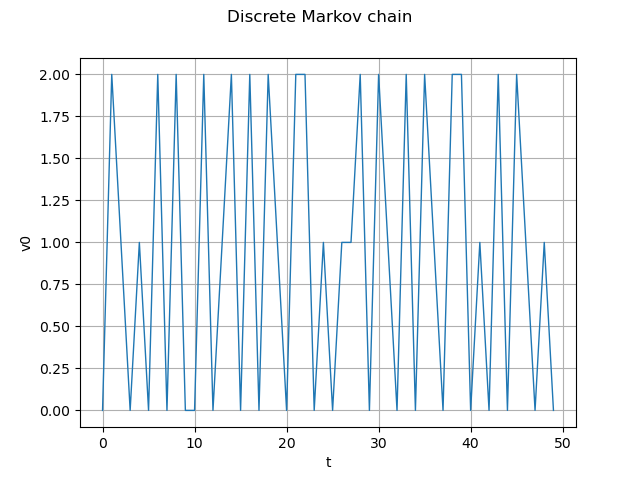
Markov chain definition and realization
process = ot.DiscreteMarkovChain(origin, transition, tgrid)
real = process.getRealization()
graph = real.drawMarginal(0)
graph.setTitle("Discrete Markov chain")
view = viewer.View(graph)
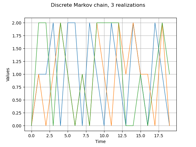
Get several realizations
process.setTimeGrid(ot.RegularGrid(0.0, 1.0, 20))
reals = process.getSample(3)
graph = reals.drawMarginal(0)
graph.setTitle("Discrete Markov chain, 3 realizations")
view = viewer.View(graph)
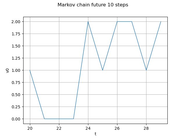
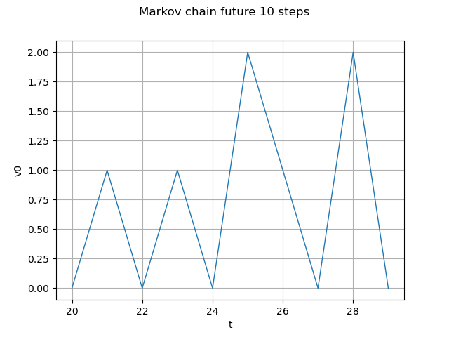
Markov chain future 10 steps
future = process.getFuture(10)
graph = future.drawMarginal(0)
graph.setTitle("Markov chain future 10 steps")
view = viewer.View(graph)
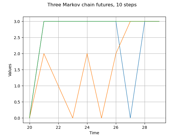
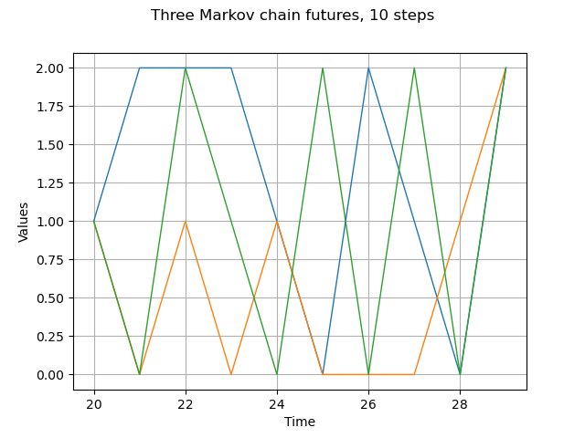
Markov chain 3 different futures
futures = process.getFuture(10, 3)
graph = futures.drawMarginal(0)
graph.setTitle("Three Markov chain futures, 10 steps")
view = viewer.View(graph)
plt.show()