Note
Go to the end to download the full example code.
Create a process from random vectors and processes
The objective is to create a process defined from a random vector and a process.
We consider the following limit state function, defined as the difference between a degrading resistance  and a time-varying load
  :
:

We propose the following probabilistic model:
 is the initial resistance, and
  ;
; is the deterioration rate of the resistance; it is deterministic;
- is the time-varying stress, which is modeled by a stationary Gaussian process of mean value
 ,
standard deviation
,
standard deviation  and a squared exponential covariance model;
  is the time, varying in
 ![[0,T]](data:image/svg+xml;base64,PD94bWwgdmVyc2lvbj0nMS4wJyBlbmNvZGluZz0nVVRGLTgnPz4KPCEtLSBUaGlzIGZpbGUgd2FzIGdlbmVyYXRlZCBieSBkdmlzdmdtIDMuNC4yIC0tPgo8c3ZnIHZlcnNpb249JzEuMScgeG1sbnM9J2h0dHA6Ly93d3cudzMub3JnLzIwMDAvc3ZnJyB4bWxuczp4bGluaz0naHR0cDovL3d3dy53My5vcmcvMTk5OS94bGluaycgd2lkdGg9JzI2LjA4NzMwN3B0JyBoZWlnaHQ9JzExLjk1NTE2OHB0JyB2aWV3Qm94PScwIC04Ljk2NjM3NiAyNi4wODczMDcgMTEuOTU1MTY4Jz4KPGRlZnM+CjxwYXRoIGlkPSdnMC01OScgZD0nTTIuMzMxMjU4IC4wNDc4MjFDMi4zMzEyNTgtLjY0NTU3OSAyLjEwNDExLTEuMTU5NjUxIDEuNjEzOTQ4LTEuMTU5NjUxQzEuMjMxMzgyLTEuMTU5NjUxIDEuMDQwMS0uODQ4ODE3IDEuMDQwMS0uNTg1ODAzUzEuMjE5NDI3IDAgMS42MjU5MDMgMEMxLjc4MTMyIDAgMS45MTI4MjctLjA0NzgyMSAyLjAyMDQyMy0uMTU1NDE3QzIuMDQ0MzM0LS4xNzkzMjggMi4wNTYyODktLjE3OTMyOCAyLjA2ODI0NC0uMTc5MzI4QzIuMDkyMTU0LS4xNzkzMjggMi4wOTIxNTQtLjAxMTk1NSAyLjA5MjE1NCAuMDQ3ODIxQzIuMDkyMTU0IC40NDIzNDEgMi4wMjA0MjMgMS4yMTk0MjcgMS4zMjcwMjQgMS45OTY1MTNDMS4xOTU1MTcgMi4xMzk5NzUgMS4xOTU1MTcgMi4xNjM4ODUgMS4xOTU1MTcgMi4xODc3OTZDMS4xOTU1MTcgMi4yNDc1NzIgMS4yNTUyOTMgMi4zMDczNDcgMS4zMTUwNjggMi4zMDczNDdDMS40MTA3MSAyLjMwNzM0NyAyLjMzMTI1OCAxLjQyMjY2NSAyLjMzMTI1OCAuMDQ3ODIxWicvPgo8cGF0aCBpZD0nZzAtODQnIGQ9J000Ljk4NTMwNS03LjI5MjY1M0M1LjA1NzAzNi03LjU3OTU3NyA1LjA4MDk0Ni03LjY4NzE3MyA1LjI2MDI3NC03LjczNDk5NEM1LjM1NTkxNS03Ljc1ODkwNCA1Ljc1MDQzNi03Ljc1ODkwNCA2LjAwMTQ5NC03Ljc1ODkwNEM3LjE5NzAxMS03Ljc1ODkwNCA3Ljc1ODkwNC03LjcxMTA4MyA3Ljc1ODkwNC02Ljc3ODU4QzcuNzU4OTA0LTYuNTk5MjUzIDcuNzExMDgzLTYuMTQ0OTU2IDcuNjM5MzUyLTUuNzAyNjE1TDcuNjI3Mzk3LTUuNTU5MTUzQzcuNjI3Mzk3LTUuNTExMzMzIDcuNjc1MjE4LTUuNDM5NjAxIDcuNzQ2OTQ5LTUuNDM5NjAxQzcuODY2NTAxLTUuNDM5NjAxIDcuODY2NTAxLTUuNDk5Mzc3IDcuOTAyMzY2LTUuNjkwNjZMOC4yNDkwNjYtNy44MDY3MjVDOC4yNzI5NzYtNy45MTQzMjEgOC4yNzI5NzYtNy45MzgyMzIgOC4yNzI5NzYtNy45NzQwOTdDOC4yNzI5NzYtOC4xMDU2MDQgOC4yMDEyNDUtOC4xMDU2MDQgNy45NjIxNDItOC4xMDU2MDRIMS40MjI2NjVDMS4xNDc2OTYtOC4xMDU2MDQgMS4xMzU3NDEtOC4wOTM2NDkgMS4wNjQwMS03Ljg3ODQ1NkwuMzM0NzQ1LTUuNzI2NTI2Qy4zMjI3OS01LjcwMjYxNSAuMjg2OTI0LTUuNTcxMTA4IC4yODY5MjQtNS41NTkxNTNDLjI4NjkyNC01LjQ5OTM3NyAuMzM0NzQ1LTUuNDM5NjAxIC40MDY0NzYtNS40Mzk2MDFDLjUwMjExNy01LjQzOTYwMSAuNTI2MDI3LTUuNDg3NDIyIC41NzM4NDgtNS42NDI4MzlDMS4wNzU5NjUtNy4wODk0MTUgMS4zMjcwMjQtNy43NTg5MDQgMi45MTcwNjEtNy43NTg5MDRIMy43MTgwNTdDNC4wMDQ5ODEtNy43NTg5MDQgNC4xMjQ1MzMtNy43NTg5MDQgNC4xMjQ1MzMtNy42MjczOTdDNC4xMjQ1MzMtNy41OTE1MzIgNC4xMjQ1MzMtNy41Njc2MjEgNC4wNjQ3NTctNy4zNTI0MjhMMi40NjI3NjUtLjkzMjUwM0MyLjM0MzIxMy0uNDY2MjUyIDIuMzE5MzAzLS4zNDY3IDEuMDUyMDU1LS4zNDY3Qy43NTMxNzYtLjM0NjcgLjY2OTQ4OS0uMzQ2NyAuNjY5NDg5LS4xMTk1NTJDLjY2OTQ4OSAwIC44MDA5OTYgMCAuODYwNzcyIDBDMS4xNTk2NTEgMCAxLjQ3MDQ4Ni0uMDIzOTEgMS43NjkzNjUtLjAyMzkxSDMuNjM0MzcxQzMuOTMzMjUtLjAyMzkxIDQuMjU2MDQgMCA0LjU1NDkxOSAwQzQuNjg2NDI2IDAgNC44MDU5NzggMCA0LjgwNTk3OC0uMjI3MTQ4QzQuODA1OTc4LS4zNDY3IDQuNzIyMjkxLS4zNDY3IDQuNDExNDU3LS4zNDY3QzMuMzM1NDkyLS4zNDY3IDMuMzM1NDkyLS40NTQyOTYgMy4zMzU0OTItLjYzMzYyNEMzLjMzNTQ5Mi0uNjQ1NTc5IDMuMzM1NDkyLS43MjkyNjUgMy4zODMzMTMtLjkyMDU0OEw0Ljk4NTMwNS03LjI5MjY1M1onLz4KPHBhdGggaWQ9J2cxLTQ4JyBkPSdNNS4zNTU5MTUtMy44MjU2NTRDNS4zNTU5MTUtNC44MTc5MzMgNS4yOTYxMzktNS43ODYzMDEgNC44NjU3NTMtNi42OTQ4OTRDNC4zNzU1OTItNy42ODcxNzMgMy41MTQ4MTktNy45NTAxODcgMi45MjkwMTYtNy45NTAxODdDMi4yMzU2MTYtNy45NTAxODcgMS4zODY4LTcuNjAzNDg3IC45NDQ0NTgtNi42MTEyMDhDLjYwOTcxNC01Ljg1ODAzMiAuNDkwMTYyLTUuMTE2ODEyIC40OTAxNjItMy44MjU2NTRDLjQ5MDE2Mi0yLjY2NjAwMiAuNTczODQ4LTEuNzkzMjc1IDEuMDA0MjM0LS45NDQ0NThDMS40NzA0ODYtLjAzNTg2NiAyLjI5NTM5MiAuMjUxMDU5IDIuOTE3MDYxIC4yNTEwNTlDMy45NTcxNjEgLjI1MTA1OSA0LjU1NDkxOS0uMzcwNjEgNC45MDE2MTktMS4wNjQwMUM1LjMzMjAwNS0xLjk2MDY0OCA1LjM1NTkxNS0zLjEzMjI1NCA1LjM1NTkxNS0zLjgyNTY1NFpNMi45MTcwNjEgLjAxMTk1NUMyLjUzNDQ5NiAuMDExOTU1IDEuNzU3NDEtLjIwMzIzOCAxLjUzMDI2Mi0xLjUwNjM1MUMxLjM5ODc1NS0yLjIyMzY2MSAxLjM5ODc1NS0zLjEzMjI1NCAxLjM5ODc1NS0zLjk2OTExNkMxLjM5ODc1NS00Ljk0OTQ0IDEuMzk4NzU1LTUuODM0MTIyIDEuNTkwMDM3LTYuNTM5NDc3QzEuNzkzMjc1LTcuMzQwNDczIDIuNDAyOTg5LTcuNzExMDgzIDIuOTE3MDYxLTcuNzExMDgzQzMuMzcxMzU3LTcuNzExMDgzIDQuMDY0NzU3LTcuNDM2MTE1IDQuMjkxOTA1LTYuNDA3OTdDNC40NDczMjMtNS43MjY1MjYgNC40NDczMjMtNC43ODIwNjcgNC40NDczMjMtMy45NjkxMTZDNC40NDczMjMtMy4xNjgxMiA0LjQ0NzMyMy0yLjI1OTUyNyA0LjMxNTgxNi0xLjUzMDI2MkM0LjA4ODY2Ny0uMjE1MTkzIDMuMzM1NDkyIC4wMTE5NTUgMi45MTcwNjEgLjAxMTk1NVonLz4KPHBhdGggaWQ9J2cxLTkxJyBkPSdNMi45ODg3OTIgMi45ODg3OTJWMi41NDY0NTFIMS44MjkxNDFWLTguNTI0MDM1SDIuOTg4NzkyVi04Ljk2NjM3NkgxLjM4NjhWMi45ODg3OTJIMi45ODg3OTJaJy8+CjxwYXRoIGlkPSdnMS05MycgZD0nTTEuODUzMDUxLTguOTY2Mzc2SC4yNTEwNTlWLTguNTI0MDM1SDEuNDEwNzFWMi41NDY0NTFILjI1MTA1OVYyLjk4ODc5MkgxLjg1MzA1MVYtOC45NjYzNzZaJy8+CjwvZGVmcz4KPGcgaWQ9J3BhZ2UxJz4KPHVzZSB4PScwJyB5PScwJyB4bGluazpocmVmPScjZzEtOTEnLz4KPHVzZSB4PSczLjI1MTY2MScgeT0nMCcgeGxpbms6aHJlZj0nI2cxLTQ4Jy8+Cjx1c2UgeD0nOS4xMDQ2NTInIHk9JzAnIHhsaW5rOmhyZWY9JyNnMC01OScvPgo8dXNlIHg9JzE0LjM0ODgxJyB5PScwJyB4bGluazpocmVmPScjZzAtODQnLz4KPHVzZSB4PScyMi44MzU2NDYnIHk9JzAnIHhsaW5rOmhyZWY9JyNnMS05MycvPgo8L2c+Cjwvc3ZnPgo8IS0tIERFUFRIPTQgLS0+) .
.
First, import the python modules:
import openturns as ot
from openturns.viewer import View
import math as m
1. Create the Gaussian process  
Create the mesh which is a regular grid on , with  , by step =1:
b = 0.01
t0 = 0.0
step = 1
tfin = 50
n = round((tfin - t0) / step)
myMesh = ot.RegularGrid(t0, step, n)
Create the squared exponential covariance model:

where the scale parameter is  and the amplitude
  .
.
ll = 10 / m.sqrt(2)
myCovKernel = ot.SquaredExponential([ll])
print("cov model = ", myCovKernel)
cov model = SquaredExponential(scale=[7.07107], amplitude=[1])
Create the Gaussian process :
S_proc = ot.GaussianProcess(myCovKernel, myMesh)
2. Create the process  
First, create the random variable , with  and
and  :
:
muR = 5
sigR = 0.3
R = ot.Normal(muR, sigR)
The create the Dirac random variable  :
:
B = ot.Dirac(b)
Then create the process using the FunctionalBasisProcess class
and the functional basis  and
and  :
:

with  independent.
const_func = ot.SymbolicFunction(["t"], ["1"])
linear_func = ot.SymbolicFunction(["t"], ["-t"])
myBasis = ot.Basis([const_func, linear_func])

coef = ot.JointDistribution([R, B])

R_proc = ot.FunctionalBasisProcess(coef, myBasis, myMesh)
3. Create the process  
First, aggregate both processes into one process of dimension 2: 
myRS_proc = ot.AggregatedProcess([R_proc, S_proc])
Then create the spatial field function that acts only on the values of the process, keeping the mesh unchanged, using the ValueFunction class.
We define the function  on
on  by:
by:

in order to define the spatial field function  that acts on fields, defined by:
![\forall t\in [0,T], g_{dyn}(X(\omega, t), Y(\omega, t)) = X(\omega, t) - Y(\omega, t)](data:image/svg+xml;base64,PD94bWwgdmVyc2lvbj0nMS4wJyBlbmNvZGluZz0nVVRGLTgnPz4KPCEtLSBUaGlzIGZpbGUgd2FzIGdlbmVyYXRlZCBieSBkdmlzdmdtIDMuNC4yIC0tPgo8c3ZnIHZlcnNpb249JzEuMScgeG1sbnM9J2h0dHA6Ly93d3cudzMub3JnLzIwMDAvc3ZnJyB4bWxuczp4bGluaz0naHR0cDovL3d3dy53My5vcmcvMTk5OS94bGluaycgd2lkdGg9JzI2Ni44NjMwMzdwdCcgaGVpZ2h0PScxMi4zMDkzODVwdCcgdmlld0JveD0nNjAuODQwMDExIC0xMy4zNTAwMjMgMjY2Ljg2MzAzNyAxMi4zMDkzODUnPgo8ZGVmcz4KPHBhdGggaWQ9J2cxLTEwMCcgZD0nTTQuMjg3OTItNS4yOTIxNTRDNC4yOTU4OS01LjMwODA5NSA0LjMxOTgwMS01LjQxMTcwNiA0LjMxOTgwMS01LjQxOTY3NkM0LjMxOTgwMS01LjQ1OTUyNyA0LjI4NzkyLTUuNTMxMjU4IDQuMTkyMjc5LTUuNTMxMjU4QzQuMTYwMzk5LTUuNTMxMjU4IDMuOTEzMzI1LTUuNTA3MzQ3IDMuNzMwMDEyLTUuNDkxNDA3TDMuMjgzNjg2LTUuNDU5NTI3QzMuMTA4MzQ0LTUuNDQzNTg3IDMuMDI4NjQzLTUuNDM1NjE2IDMuMDI4NjQzLTUuMjkyMTU0QzMuMDI4NjQzLTUuMTgwNTczIDMuMTQwMjI0LTUuMTgwNTczIDMuMjM1ODY2LTUuMTgwNTczQzMuNjE4NDMxLTUuMTgwNTczIDMuNjE4NDMxLTUuMTMyNzUyIDMuNjE4NDMxLTUuMDYxMDIxQzMuNjE4NDMxLTUuMDEzMiAzLjU1NDY3LTQuNzUwMTg3IDMuNTE0ODE5LTQuNTkwNzg1TDMuMTI0Mjg0LTMuMDM2NjEzQzMuMDUyNTUzLTMuMTcyMTA1IDIuODIxNDItMy41MTQ4MTkgMi4zMzUyNDMtMy41MTQ4MTlDMS4zODY4LTMuNTE0ODE5IC4zNDI3MTUtMi40MDY5NzQgLjM0MjcxNS0xLjIyNzM5N0MuMzQyNzE1LS4zOTg1MDYgLjg3NjcxMiAuMDc5NzAxIDEuNDkwNDExIC4wNzk3MDFDMi4wMDA0OTggLjA3OTcwMSAyLjQzODg1NC0uMzI2Nzc1IDIuNTgyMzE2LS40ODYxNzdDMi43MjU3NzggLjA2Mzc2MSAzLjI2Nzc0NiAuMDc5NzAxIDMuMzYzMzg3IC4wNzk3MDFDMy43MzAwMTIgLjA3OTcwMSAzLjkxMzMyNS0uMjIzMTYzIDMuOTc3MDg2LS4zNTg2NTVDNC4xMzY0ODgtLjY0NTU3OSA0LjI0ODA3LTEuMTA3ODQ2IDQuMjQ4MDctMS4xMzk3MjZDNC4yNDgwNy0xLjE4NzU0NyA0LjIxNjE4OS0xLjI0MzMzNyA0LjEyMDU0OC0xLjI0MzMzN1M0LjAwODk2Ni0xLjE5NTUxNyAzLjk2MTE0Ni0uOTk2MjY0QzMuODQ5NTY0LS41NTc5MDggMy42OTgxMzItLjE0MzQ2MiAzLjM4NzI5OC0uMTQzNDYyQzMuMjAzOTg1LS4xNDM0NjIgMy4xMzIyNTQtLjI5NDg5NCAzLjEzMjI1NC0uNTE4MDU3QzMuMTMyMjU0LS42Njk0ODkgMy4xNTYxNjQtLjc1NzE2MSAzLjE4MDA3NS0uODYwNzcyTDQuMjg3OTItNS4yOTIxNTRaTTIuNTgyMzE2LS44NjA3NzJDMi4xODM4MTEtLjMxMDgzNCAxLjc2OTM2NS0uMTQzNDYyIDEuNTE0MzIxLS4xNDM0NjJDMS4xNDc2OTYtLjE0MzQ2MiAuOTY0Mzg0LS40NzgyMDcgLjk2NDM4NC0uODkyNjUzQy45NjQzODQtMS4yNjcyNDggMS4xNzk1NzctMi4xMjAwNSAxLjM1NDkxOS0yLjQ3MDczNUMxLjU4NjA1Mi0yLjk1NjkxMiAxLjk3NjU4OC0zLjI5MTY1NiAyLjM0MzIxMy0zLjI5MTY1NkMyLjg2MTI3LTMuMjkxNjU2IDMuMDEyNzAyLTIuNzA5ODM4IDMuMDEyNzAyLTIuNjE0MTk3QzMuMDEyNzAyLTIuNTgyMzE2IDIuODEzNDUtMS44MDEyNDUgMi43NjU2MjktMS41OTQwMjJDMi42NjIwMTctMS4yMTk0MjcgMi42NjIwMTctMS4yMDM0ODcgMi41ODIzMTYtLjg2MDc3MlonLz4KPHBhdGggaWQ9J2cxLTExMCcgZD0nTTEuNTk0MDIyLTEuMzA3MDk4QzEuNjE3OTMzLTEuNDI2NjUgMS42OTc2MzQtMS43Mjk1MTQgMS43MjE1NDQtMS44NDkwNjZDMS44MzMxMjYtMi4yNzk0NTIgMS44MzMxMjYtMi4yODc0MjIgMi4wMTY0MzgtMi41NTA0MzZDMi4yNzk0NTItMi45NDA5NzEgMi42NTQwNDctMy4yOTE2NTYgMy4xODgwNDUtMy4yOTE2NTZDMy40NzQ5NjktMy4yOTE2NTYgMy42NDIzNDEtMy4xMjQyODQgMy42NDIzNDEtMi43NDk2ODlDMy42NDIzNDEtMi4zMTEzMzMgMy4zMDc1OTctMS40MDI3NCAzLjE1NjE2NC0xLjAxMjIwNEMzLjA1MjU1My0uNzQ5MTkxIDMuMDUyNTUzLS43MDEzNyAzLjA1MjU1My0uNTk3NzU4QzMuMDUyNTUzLS4xNDM0NjIgMy40MjcxNDggLjA3OTcwMSAzLjc2OTg2MyAuMDc5NzAxQzQuNTUwOTM0IC4wNzk3MDEgNC44Nzc3MDktMS4wMzYxMTUgNC44Nzc3MDktMS4xMzk3MjZDNC44Nzc3MDktMS4yMTk0MjcgNC44MTM5NDgtMS4yNDMzMzcgNC43NTgxNTctMS4yNDMzMzdDNC42NjI1MTYtMS4yNDMzMzcgNC42NDY1NzUtMS4xODc1NDcgNC42MjI2NjUtMS4xMDc4NDZDNC40MzEzODItLjQ1NDI5NiA0LjA5NjYzOC0uMTQzNDYyIDMuNzkzNzczLS4xNDM0NjJDMy42NjYyNTItLjE0MzQ2MiAzLjYwMjQ5MS0uMjIzMTYzIDMuNjAyNDkxLS40MDY0NzZTMy42NjYyNTItLjc2NTEzMSAzLjc0NTk1My0uOTY0Mzg0QzMuODY1NTA0LTEuMjY3MjQ4IDQuMjE2MTg5LTIuMTgzODExIDQuMjE2MTg5LTIuNjMwMTM3QzQuMjE2MTg5LTMuMjI3ODk1IDMuODAxNzQzLTMuNTE0ODE5IDMuMjI3ODk1LTMuNTE0ODE5QzIuNTgyMzE2LTMuNTE0ODE5IDIuMTY3ODctMy4xMjQyODQgMS45MzY3MzctMi44MjE0MkMxLjg4MDk0Ni0zLjI1OTc3NiAxLjUzMDI2Mi0zLjUxNDgxOSAxLjEyMzc4Ni0zLjUxNDgxOUMuODM2ODYyLTMuNTE0ODE5IC42Mzc2MDktMy4zMzE1MDcgLjUxMDA4Ny0zLjA4NDQzM0MuMzE4ODA0LTIuNzA5ODM4IC4yMzkxMDMtMi4zMTEzMzMgLjIzOTEwMy0yLjI5NTM5MkMuMjM5MTAzLTIuMjIzNjYxIC4yOTQ4OTQtMi4xOTE3ODEgLjM1ODY1NS0yLjE5MTc4MUMuNDYyMjY3LTIuMTkxNzgxIC40NzAyMzctMi4yMjM2NjEgLjUyNjAyNy0yLjQzMDg4NEMuNjIxNjY5LTIuODIxNDIgLjc2NTEzMS0zLjI5MTY1NiAxLjA5OTg3NS0zLjI5MTY1NkMxLjMwNzA5OC0zLjI5MTY1NiAxLjM1NDkxOS0zLjA5MjQwMyAxLjM1NDkxOS0yLjkxNzA2MUMxLjM1NDkxOS0yLjc3MzU5OSAxLjMxNTA2OC0yLjYyMjE2NyAxLjI1MTMwOC0yLjM1OTE1M0MxLjIzNTM2Ny0yLjI5NTM5MiAxLjExNTgxNi0xLjgyNTE1NiAxLjA4MzkzNS0xLjcxMzU3NEwuNzg5MDQxLS41MTgwNTdDLjc1NzE2MS0uMzk4NTA2IC43MDkzNC0uMTk5MjUzIC43MDkzNC0uMTY3MzcyQy43MDkzNCAuMDE1OTQgLjg2MDc3MiAuMDc5NzAxIC45NjQzODQgLjA3OTcwMUMxLjEwNzg0NiAuMDc5NzAxIDEuMjI3Mzk3LS4wMTU5NCAxLjI4MzE4OC0uMTExNTgyQzEuMzA3MDk4LS4xNTk0MDIgMS4zNzA4NTktLjQzMDM4NiAxLjQxMDcxLS41OTc3NThMMS41OTQwMjItMS4zMDcwOThaJy8+CjxwYXRoIGlkPSdnMS0xMjEnIGQ9J000LjEyODUxOC0zLjAwNDczMkM0LjE2MDM5OS0zLjExNjMxNCA0LjE2MDM5OS0zLjEzMjI1NCA0LjE2MDM5OS0zLjE4ODA0NUM0LjE2MDM5OS0zLjM4NzI5OCA0LjAwMDk5Ni0zLjQzNTExOCAzLjkwNTM1NS0zLjQzNTExOEMzLjg2NTUwNC0zLjQzNTExOCAzLjY4MjE5Mi0zLjQyNzE0OCAzLjU3ODU4LTMuMjE5OTI1QzMuNTYyNjQtMy4xODAwNzUgMy40OTA5MDktMi44OTMxNTEgMy40NTEwNTktMi43MjU3NzhMMi45NzI4NTItLjgxMjk1MUMyLjk2NDg4Mi0uNzg5MDQxIDIuNjIyMTY3LS4xNDM0NjIgMi4wNDAzNDktLjE0MzQ2MkMxLjY0OTgxMy0uMTQzNDYyIDEuNTE0MzIxLS40MzAzODYgMS41MTQzMjEtLjc4OTA0MUMxLjUxNDMyMS0xLjI1MTMwOCAxLjc4NTMwNS0xLjk2MDY0OCAxLjk2ODYxOC0yLjQyMjkxNEMyLjA0ODMxOS0yLjYyMjE2NyAyLjA3MjIyOS0yLjY5Mzg5OCAyLjA3MjIyOS0yLjgzNzM2QzIuMDcyMjI5LTMuMjc1NzE2IDEuNzIxNTQ0LTMuNTE0ODE5IDEuMzU0OTE5LTMuNTE0ODE5Qy41NjU4NzgtMy41MTQ4MTkgLjIzOTEwMy0yLjM5MTAzNCAuMjM5MTAzLTIuMjk1MzkyQy4yMzkxMDMtMi4yMjM2NjEgLjI5NDg5NC0yLjE5MTc4MSAuMzU4NjU1LTIuMTkxNzgxQy40NjIyNjctMi4xOTE3ODEgLjQ3MDIzNy0yLjIzOTYwMSAuNDk0MTQ3LTIuMzE5MzAzQy43MDEzNy0zLjAxMjcwMiAxLjA0NDA4NS0zLjI5MTY1NiAxLjMzMTAwOS0zLjI5MTY1NkMxLjQ1MDU2LTMuMjkxNjU2IDEuNTIyMjkxLTMuMjExOTU1IDEuNTIyMjkxLTMuMDI4NjQzQzEuNTIyMjkxLTIuODYxMjcgMS40NTg1MzEtMi42Nzc5NTggMS40MDI3NC0yLjUzNDQ5NkMxLjA3NTk2NS0xLjY4OTY2NCAuOTQwNDczLTEuMjgzMTg4IC45NDA0NzMtLjkwODU5M0MuOTQwNDczLS4xMjc1MjIgMS41MzAyNjIgLjA3OTcwMSAyLjAwMDQ5OCAuMDc5NzAxQzIuMzc1MDkzIC4wNzk3MDEgMi42NDYwNzctLjA4NzY3MSAyLjgzNzM2LS4yNzA5ODRDMi43MjU3NzggLjE3NTM0MiAyLjY0NjA3NyAuNDg2MTc3IDIuMzQzMjEzIC44Njg3NDJDMi4wODAxOTkgMS4xOTU1MTcgMS43NjEzOTUgMS40MDI3NCAxLjQwMjc0IDEuNDAyNzRDMS4yNjcyNDggMS40MDI3NCAuOTY0Mzg0IDEuMzc4ODI5IC44MDQ5ODEgMS4xMzk3MjZDMS4yMjczOTcgMS4xMDc4NDYgMS4yNTkyNzggLjc0OTE5MSAxLjI1OTI3OCAuNzAxMzdDMS4yNTkyNzggLjUxMDA4NyAxLjExNTgxNiAuNDA2NDc2IC45NDg0NDMgLjQwNjQ3NkMuNzczMTAxIC40MDY0NzYgLjQ5NDE0NyAuNTQxOTY4IC40OTQxNDcgLjkzMjUwM0MuNDk0MTQ3IDEuMzA3MDk4IC44MzY4NjIgMS42MjU5MDMgMS40MDI3NCAxLjYyNTkwM0MyLjIxNTY5MSAxLjYyNTkwMyAzLjEzMjI1NCAuOTcyMzU0IDMuMzcxMzU3IC4wMDc5N0w0LjEyODUxOC0zLjAwNDczMlonLz4KPHBhdGggaWQ9J2czLTQwJyBkPSdNMy44ODU0MyAyLjkwNTEwNkMzLjg4NTQzIDIuODY5MjQgMy44ODU0MyAyLjg0NTMzIDMuNjgyMTkyIDIuNjQyMDkyQzIuNDg2Njc1IDEuNDM0NjIgMS44MTcxODYtLjUzNzk4MyAxLjgxNzE4Ni0yLjk3NjgzN0MxLjgxNzE4Ni01LjI5NjEzOSAyLjM3OTA3OC03LjI5MjY1MyAzLjc2NTg3OC04LjcwMzM2MkMzLjg4NTQzLTguODEwOTU5IDMuODg1NDMtOC44MzQ4NjkgMy44ODU0My04Ljg3MDczNUMzLjg4NTQzLTguOTQyNDY2IDMuODI1NjU0LTguOTY2Mzc2IDMuNzc3ODMzLTguOTY2Mzc2QzMuNjIyNDE2LTguOTY2Mzc2IDIuNjQyMDkyLTguMTA1NjA0IDIuMDU2Mjg5LTYuOTMzOTk4QzEuNDQ2NTc1LTUuNzI2NTI2IDEuMTcxNjA2LTQuNDQ3MzIzIDEuMTcxNjA2LTIuOTc2ODM3QzEuMTcxNjA2LTEuOTEyODI3IDEuMzM4OTc5LS40OTAxNjIgMS45NjA2NDggLjc4OTA0MUMyLjY2NjAwMiAyLjIyMzY2MSAzLjY0NjMyNiAzLjAwMDc0NyAzLjc3NzgzMyAzLjAwMDc0N0MzLjgyNTY1NCAzLjAwMDc0NyAzLjg4NTQzIDIuOTc2ODM3IDMuODg1NDMgMi45MDUxMDZaJy8+CjxwYXRoIGlkPSdnMy00MScgZD0nTTMuMzcxMzU3LTIuOTc2ODM3QzMuMzcxMzU3LTMuODg1NDMgMy4yNTE4MDYtNS4zNjc4NyAyLjU4MjMxNi02Ljc1NDY3QzEuODc2OTYxLTguMTg5MjkgLjg5NjYzOC04Ljk2NjM3NiAuNzY1MTMxLTguOTY2Mzc2Qy43MTczMS04Ljk2NjM3NiAuNjU3NTM0LTguOTQyNDY2IC42NTc1MzQtOC44NzA3MzVDLjY1NzUzNC04LjgzNDg2OSAuNjU3NTM0LTguODEwOTU5IC44NjA3NzItOC42MDc3MjFDMi4wNTYyODktNy40MDAyNDkgMi43MjU3NzgtNS40Mjc2NDYgMi43MjU3NzgtMi45ODg3OTJDMi43MjU3NzgtLjY2OTQ4OSAyLjE2Mzg4NSAxLjMyNzAyNCAuNzc3MDg2IDIuNzM3NzMzQy42NTc1MzQgMi44NDUzMyAuNjU3NTM0IDIuODY5MjQgLjY1NzUzNCAyLjkwNTEwNkMuNjU3NTM0IDIuOTc2ODM3IC43MTczMSAzLjAwMDc0NyAuNzY1MTMxIDMuMDAwNzQ3Qy45MjA1NDggMy4wMDA3NDcgMS45MDA4NzIgMi4xMzk5NzUgMi40ODY2NzUgLjk2ODM2OUMzLjA5NjM4OS0uMjUxMDU5IDMuMzcxMzU3LTEuNTQyMjE3IDMuMzcxMzU3LTIuOTc2ODM3WicvPgo8cGF0aCBpZD0nZzMtNDgnIGQ9J001LjM1NTkxNS0zLjgyNTY1NEM1LjM1NTkxNS00LjgxNzkzMyA1LjI5NjEzOS01Ljc4NjMwMSA0Ljg2NTc1My02LjY5NDg5NEM0LjM3NTU5Mi03LjY4NzE3MyAzLjUxNDgxOS03Ljk1MDE4NyAyLjkyOTAxNi03Ljk1MDE4N0MyLjIzNTYxNi03Ljk1MDE4NyAxLjM4NjgtNy42MDM0ODcgLjk0NDQ1OC02LjYxMTIwOEMuNjA5NzE0LTUuODU4MDMyIC40OTAxNjItNS4xMTY4MTIgLjQ5MDE2Mi0zLjgyNTY1NEMuNDkwMTYyLTIuNjY2MDAyIC41NzM4NDgtMS43OTMyNzUgMS4wMDQyMzQtLjk0NDQ1OEMxLjQ3MDQ4Ni0uMDM1ODY2IDIuMjk1MzkyIC4yNTEwNTkgMi45MTcwNjEgLjI1MTA1OUMzLjk1NzE2MSAuMjUxMDU5IDQuNTU0OTE5LS4zNzA2MSA0LjkwMTYxOS0xLjA2NDAxQzUuMzMyMDA1LTEuOTYwNjQ4IDUuMzU1OTE1LTMuMTMyMjU0IDUuMzU1OTE1LTMuODI1NjU0Wk0yLjkxNzA2MSAuMDExOTU1QzIuNTM0NDk2IC4wMTE5NTUgMS43NTc0MS0uMjAzMjM4IDEuNTMwMjYyLTEuNTA2MzUxQzEuMzk4NzU1LTIuMjIzNjYxIDEuMzk4NzU1LTMuMTMyMjU0IDEuMzk4NzU1LTMuOTY5MTE2QzEuMzk4NzU1LTQuOTQ5NDQgMS4zOTg3NTUtNS44MzQxMjIgMS41OTAwMzctNi41Mzk0NzdDMS43OTMyNzUtNy4zNDA0NzMgMi40MDI5ODktNy43MTEwODMgMi45MTcwNjEtNy43MTEwODNDMy4zNzEzNTctNy43MTEwODMgNC4wNjQ3NTctNy40MzYxMTUgNC4yOTE5MDUtNi40MDc5N0M0LjQ0NzMyMy01LjcyNjUyNiA0LjQ0NzMyMy00Ljc4MjA2NyA0LjQ0NzMyMy0zLjk2OTExNkM0LjQ0NzMyMy0zLjE2ODEyIDQuNDQ3MzIzLTIuMjU5NTI3IDQuMzE1ODE2LTEuNTMwMjYyQzQuMDg4NjY3LS4yMTUxOTMgMy4zMzU0OTIgLjAxMTk1NSAyLjkxNzA2MSAuMDExOTU1WicvPgo8cGF0aCBpZD0nZzMtNjEnIGQ9J004LjA2OTczOC0zLjg3MzQ3NEM4LjIzNzExMS0zLjg3MzQ3NCA4LjQ1MjMwNC0zLjg3MzQ3NCA4LjQ1MjMwNC00LjA4ODY2N0M4LjQ1MjMwNC00LjMxNTgxNiA4LjI0OTA2Ni00LjMxNTgxNiA4LjA2OTczOC00LjMxNTgxNkgxLjAyODE0NEMuODYwNzcyLTQuMzE1ODE2IC42NDU1NzktNC4zMTU4MTYgLjY0NTU3OS00LjEwMDYyM0MuNjQ1NTc5LTMuODczNDc0IC44NDg4MTctMy44NzM0NzQgMS4wMjgxNDQtMy44NzM0NzRIOC4wNjk3MzhaTTguMDY5NzM4LTEuNjQ5ODEzQzguMjM3MTExLTEuNjQ5ODEzIDguNDUyMzA0LTEuNjQ5ODEzIDguNDUyMzA0LTEuODY1MDA2QzguNDUyMzA0LTIuMDkyMTU0IDguMjQ5MDY2LTIuMDkyMTU0IDguMDY5NzM4LTIuMDkyMTU0SDEuMDI4MTQ0Qy44NjA3NzItMi4wOTIxNTQgLjY0NTU3OS0yLjA5MjE1NCAuNjQ1NTc5LTEuODc2OTYxQy42NDU1NzktMS42NDk4MTMgLjg0ODgxNy0xLjY0OTgxMyAxLjAyODE0NC0xLjY0OTgxM0g4LjA2OTczOFonLz4KPHBhdGggaWQ9J2czLTkxJyBkPSdNMi45ODg3OTIgMi45ODg3OTJWMi41NDY0NTFIMS44MjkxNDFWLTguNTI0MDM1SDIuOTg4NzkyVi04Ljk2NjM3NkgxLjM4NjhWMi45ODg3OTJIMi45ODg3OTJaJy8+CjxwYXRoIGlkPSdnMy05MycgZD0nTTEuODUzMDUxLTguOTY2Mzc2SC4yNTEwNTlWLTguNTI0MDM1SDEuNDEwNzFWMi41NDY0NTFILjI1MTA1OVYyLjk4ODc5MkgxLjg1MzA1MVYtOC45NjYzNzZaJy8+CjxwYXRoIGlkPSdnMi0zMycgZD0nTTcuMTAxMzctNC40OTUxNDNDNy4xMDEzNy00Ljg0MTg0MyA3LjAwNTcyOS01LjI4NDE4NCA2LjU4NzI5OC01LjI4NDE4NEM2LjM0ODE5NC01LjI4NDE4NCA2LjA3MzIyNS00Ljk4NTMwNSA2LjA3MzIyNS00Ljc0NjIwMkM2LjA3MzIyNS00LjYzODYwNSA2LjEyMTA0Ni00LjU2Njg3NCA2LjIxNjY4Ny00LjQ1OTI3OEM2LjM5NjAxNS00LjI1NjA0IDYuNjIzMTYzLTMuOTMzMjUgNi42MjMxNjMtMy4zNzEzNTdDNi42MjMxNjMtMi45NDA5NzEgNi4zNjAxNDktMi4yNTk1MjcgNi4xNjg4NjctMS44ODg5MTdDNS44MzQxMjItMS4yMzEzODIgNS4yODQxODQtLjY2OTQ4OSA0LjY2MjUxNi0uNjY5NDg5QzMuOTA5MzQtLjY2OTQ4OSAzLjYyMjQxNi0xLjE0NzY5NiAzLjQ5MDkwOS0xLjgxNzE4NkMzLjYyMjQxNi0yLjEyODAyIDMuODk3Mzg1LTIuOTA1MTA2IDMuODk3Mzg1LTMuMjE1OTRDMy44OTczODUtMy4zNDc0NDcgMy44NDk1NjQtMy40NTUwNDQgMy42OTQxNDctMy40NTUwNDRDMy42MTA0NjEtMy40NTUwNDQgMy41MTQ4MTktMy40MDcyMjMgMy40NTUwNDQtMy4zMTE1ODJDMy4yODc2NzEtMy4wNDg1NjggMy4xMzIyNTQtMi4xMDQxMSAzLjE0NDIwOS0xLjg1MzA1MUMyLjkxNzA2MS0xLjQxMDcxIDIuMjcxNDgyLS42Njk0ODkgMS41MDYzNTEtLjY2OTQ4OUMuNzA1MzU1LS42Njk0ODkgLjQ5MDE2Mi0xLjM3NDg0NCAuNDkwMTYyLTIuMDU2Mjg5Qy40OTAxNjItMy4yOTk2MjYgMS4yNjcyNDgtNC4zODc1NDcgMS40ODI0NDEtNC42ODY0MjZDMS42MDE5OTMtNC44NjU3NTMgMS42ODU2NzktNC45ODUzMDUgMS42ODU2NzktNS4wMDkyMTVDMS42ODU2NzktNS4wOTI5MDIgMS42Mzc4NTgtNS4yMjQ0MDggMS41MzAyNjItNS4yMjQ0MDhDMS4zMzg5NzktNS4yMjQ0MDggMS4yNzkyMDMtNS4wNjg5OTEgMS4xODM1NjItNC45MjU1MjlDLjU3Mzg0OC0zLjk4MTA3MSAuMTQzNDYyLTIuNjU0MDQ3IC4xNDM0NjItMS41MDYzNTFDLjE0MzQ2Mi0uNzY1MTMxIC40MTg0MzEgLjExOTU1MiAxLjMxNTA2OCAuMTE5NTUyQzIuMzA3MzQ3IC4xMTk1NTIgMi45MjkwMTYtLjcyOTI2NSAzLjE4MDA3NS0xLjE4MzU2MkMzLjI3NTcxNi0uNTE0MDcyIDMuNjM0MzcxIC4xMTk1NTIgNC41MDcwOTggLjExOTU1MkM1LjQxNTY5MSAuMTE5NTUyIDUuOTg5NTM5LS42ODE0NDUgNi40MTk5MjUtMS42NDk4MTNDNi43MzA3Ni0yLjM0MzIxMyA3LjEwMTM3LTMuODM3NjA5IDcuMTAxMzctNC40OTUxNDNaJy8+CjxwYXRoIGlkPSdnMi01OScgZD0nTTIuMzMxMjU4IC4wNDc4MjFDMi4zMzEyNTgtLjY0NTU3OSAyLjEwNDExLTEuMTU5NjUxIDEuNjEzOTQ4LTEuMTU5NjUxQzEuMjMxMzgyLTEuMTU5NjUxIDEuMDQwMS0uODQ4ODE3IDEuMDQwMS0uNTg1ODAzUzEuMjE5NDI3IDAgMS42MjU5MDMgMEMxLjc4MTMyIDAgMS45MTI4MjctLjA0NzgyMSAyLjAyMDQyMy0uMTU1NDE3QzIuMDQ0MzM0LS4xNzkzMjggMi4wNTYyODktLjE3OTMyOCAyLjA2ODI0NC0uMTc5MzI4QzIuMDkyMTU0LS4xNzkzMjggMi4wOTIxNTQtLjAxMTk1NSAyLjA5MjE1NCAuMDQ3ODIxQzIuMDkyMTU0IC40NDIzNDEgMi4wMjA0MjMgMS4yMTk0MjcgMS4zMjcwMjQgMS45OTY1MTNDMS4xOTU1MTcgMi4xMzk5NzUgMS4xOTU1MTcgMi4xNjM4ODUgMS4xOTU1MTcgMi4xODc3OTZDMS4xOTU1MTcgMi4yNDc1NzIgMS4yNTUyOTMgMi4zMDczNDcgMS4zMTUwNjggMi4zMDczNDdDMS40MTA3MSAyLjMwNzM0NyAyLjMzMTI1OCAxLjQyMjY2NSAyLjMzMTI1OCAuMDQ3ODIxWicvPgo8cGF0aCBpZD0nZzItODQnIGQ9J000Ljk4NTMwNS03LjI5MjY1M0M1LjA1NzAzNi03LjU3OTU3NyA1LjA4MDk0Ni03LjY4NzE3MyA1LjI2MDI3NC03LjczNDk5NEM1LjM1NTkxNS03Ljc1ODkwNCA1Ljc1MDQzNi03Ljc1ODkwNCA2LjAwMTQ5NC03Ljc1ODkwNEM3LjE5NzAxMS03Ljc1ODkwNCA3Ljc1ODkwNC03LjcxMTA4MyA3Ljc1ODkwNC02Ljc3ODU4QzcuNzU4OTA0LTYuNTk5MjUzIDcuNzExMDgzLTYuMTQ0OTU2IDcuNjM5MzUyLTUuNzAyNjE1TDcuNjI3Mzk3LTUuNTU5MTUzQzcuNjI3Mzk3LTUuNTExMzMzIDcuNjc1MjE4LTUuNDM5NjAxIDcuNzQ2OTQ5LTUuNDM5NjAxQzcuODY2NTAxLTUuNDM5NjAxIDcuODY2NTAxLTUuNDk5Mzc3IDcuOTAyMzY2LTUuNjkwNjZMOC4yNDkwNjYtNy44MDY3MjVDOC4yNzI5NzYtNy45MTQzMjEgOC4yNzI5NzYtNy45MzgyMzIgOC4yNzI5NzYtNy45NzQwOTdDOC4yNzI5NzYtOC4xMDU2MDQgOC4yMDEyNDUtOC4xMDU2MDQgNy45NjIxNDItOC4xMDU2MDRIMS40MjI2NjVDMS4xNDc2OTYtOC4xMDU2MDQgMS4xMzU3NDEtOC4wOTM2NDkgMS4wNjQwMS03Ljg3ODQ1NkwuMzM0NzQ1LTUuNzI2NTI2Qy4zMjI3OS01LjcwMjYxNSAuMjg2OTI0LTUuNTcxMTA4IC4yODY5MjQtNS41NTkxNTNDLjI4NjkyNC01LjQ5OTM3NyAuMzM0NzQ1LTUuNDM5NjAxIC40MDY0NzYtNS40Mzk2MDFDLjUwMjExNy01LjQzOTYwMSAuNTI2MDI3LTUuNDg3NDIyIC41NzM4NDgtNS42NDI4MzlDMS4wNzU5NjUtNy4wODk0MTUgMS4zMjcwMjQtNy43NTg5MDQgMi45MTcwNjEtNy43NTg5MDRIMy43MTgwNTdDNC4wMDQ5ODEtNy43NTg5MDQgNC4xMjQ1MzMtNy43NTg5MDQgNC4xMjQ1MzMtNy42MjczOTdDNC4xMjQ1MzMtNy41OTE1MzIgNC4xMjQ1MzMtNy41Njc2MjEgNC4wNjQ3NTctNy4zNTI0MjhMMi40NjI3NjUtLjkzMjUwM0MyLjM0MzIxMy0uNDY2MjUyIDIuMzE5MzAzLS4zNDY3IDEuMDUyMDU1LS4zNDY3Qy43NTMxNzYtLjM0NjcgLjY2OTQ4OS0uMzQ2NyAuNjY5NDg5LS4xMTk1NTJDLjY2OTQ4OSAwIC44MDA5OTYgMCAuODYwNzcyIDBDMS4xNTk2NTEgMCAxLjQ3MDQ4Ni0uMDIzOTEgMS43NjkzNjUtLjAyMzkxSDMuNjM0MzcxQzMuOTMzMjUtLjAyMzkxIDQuMjU2MDQgMCA0LjU1NDkxOSAwQzQuNjg2NDI2IDAgNC44MDU5NzggMCA0LjgwNTk3OC0uMjI3MTQ4QzQuODA1OTc4LS4zNDY3IDQuNzIyMjkxLS4zNDY3IDQuNDExNDU3LS4zNDY3QzMuMzM1NDkyLS4zNDY3IDMuMzM1NDkyLS40NTQyOTYgMy4zMzU0OTItLjYzMzYyNEMzLjMzNTQ5Mi0uNjQ1NTc5IDMuMzM1NDkyLS43MjkyNjUgMy4zODMzMTMtLjkyMDU0OEw0Ljk4NTMwNS03LjI5MjY1M1onLz4KPHBhdGggaWQ9J2cyLTg4JyBkPSdNNS42Nzg3MDUtNC44NTM3OThMNC41NTQ5MTktNy40NzE5OEM0LjcxMDMzNi03Ljc1ODkwNCA1LjA2ODk5MS03LjgwNjcyNSA1LjIxMjQ1My03LjgxODY4QzUuMjg0MTg0LTcuODE4NjggNS40MTU2OTEtNy44MzA2MzUgNS40MTU2OTEtOC4wMzM4NzNDNS40MTU2OTEtOC4xNjUzOCA1LjMwODA5NS04LjE2NTM4IDUuMjM2MzY0LTguMTY1MzhDNS4wMzMxMjYtOC4xNjUzOCA0Ljc5NDAyMi04LjE0MTQ2OSA0LjU5MDc4NS04LjE0MTQ2OUgzLjg5NzM4NUMzLjE2ODEyLTguMTQxNDY5IDIuNjQyMDkyLTguMTY1MzggMi42MzAxMzctOC4xNjUzOEMyLjUzNDQ5Ni04LjE2NTM4IDIuNDE0OTQ0LTguMTY1MzggMi40MTQ5NDQtNy45MzgyMzJDMi40MTQ5NDQtNy44MTg2OCAyLjUyMjU0LTcuODE4NjggMi42Nzc5NTgtNy44MTg2OEMzLjM3MTM1Ny03LjgxODY4IDMuNDE5MTc4LTcuNjk5MTI4IDMuNTM4NzMtNy40MTIyMDRMNC45NjEzOTUtNC4wODg2NjdMMi4zNjcxMjMtMS4zMTUwNjhDMS45MzY3MzctLjg0ODgxNyAxLjQyMjY2NS0uMzk0NTIxIC41Mzc5ODMtLjM0NjdDLjM5NDUyMS0uMzM0NzQ1IC4yOTg4NzktLjMzNDc0NSAuMjk4ODc5LS4xMTk1NTJDLjI5ODg3OS0uMDgzNjg2IC4zMTA4MzQgMCAuNDQyMzQxIDBDLjYwOTcxNCAwIC43ODkwNDEtLjAyMzkxIC45NTY0MTMtLjAyMzkxSDEuNTE4MzA2QzEuOTAwODcyLS4wMjM5MSAyLjMxOTMwMyAwIDIuNjg5OTEzIDBDMi43NzM1OTkgMCAyLjkxNzA2MSAwIDIuOTE3MDYxLS4yMTUxOTNDMi45MTcwNjEtLjMzNDc0NSAyLjgzMzM3NS0uMzQ2NyAyLjc2MTY0NC0uMzQ2N0MyLjUyMjU0LS4zNzA2MSAyLjM2NzEyMy0uNTAyMTE3IDIuMzY3MTIzLS42OTM0QzIuMzY3MTIzLS44OTY2MzggMi41MTA1ODUtMS4wNDAxIDIuODU3Mjg1LTEuMzk4NzU1TDMuOTIxMjk1LTIuNTU4NDA2QzQuMTg0MzA5LTIuODMzMzc1IDQuODE3OTMzLTMuNTI2Nzc1IDUuMDgwOTQ2LTMuNzg5Nzg4TDYuMzM2MjM5LS44NDg4MTdDNi4zNDgxOTQtLjgyNDkwNyA2LjM5NjAxNS0uNzA1MzU1IDYuMzk2MDE1LS42OTM0QzYuMzk2MDE1LS41ODU4MDMgNi4xMzMwMDEtLjM3MDYxIDUuNzUwNDM2LS4zNDY3QzUuNjc4NzA1LS4zNDY3IDUuNTQ3MTk4LS4zMzQ3NDUgNS41NDcxOTgtLjExOTU1MkM1LjU0NzE5OCAwIDUuNjY2NzUgMCA1LjcyNjUyNiAwQzUuOTI5NzYzIDAgNi4xNjg4NjctLjAyMzkxIDYuMzcyMTA1LS4wMjM5MUg3LjY4NzE3M0M3LjkwMjM2Ni0uMDIzOTEgOC4xMjk1MTQgMCA4LjMzMjc1MiAwQzguNDE2NDM4IDAgOC41NDc5NDUgMCA4LjU0Nzk0NS0uMjI3MTQ4QzguNTQ3OTQ1LS4zNDY3IDguNDI4Mzk0LS4zNDY3IDguMzIwNzk3LS4zNDY3QzcuNjAzNDg3LS4zNTg2NTUgNy41Nzk1NzctLjQxODQzMSA3LjM3NjMzOS0uODYwNzcyTDUuNzk4MjU3LTQuNTY2ODc0TDcuMzE2NTYzLTYuMTkyNzc3QzcuNDM2MTE1LTYuMzEyMzI5IDcuNzExMDgzLTYuNjExMjA4IDcuODE4NjgtNi43MzA3NkM4LjMzMjc1Mi03LjI2ODc0MiA4LjgxMDk1OS03Ljc1ODkwNCA5Ljc3OTMyOC03LjgxODY4QzkuODk4ODc5LTcuODMwNjM1IDEwLjAxODQzMS03LjgzMDYzNSAxMC4wMTg0MzEtOC4wMzM4NzNDMTAuMDE4NDMxLTguMTY1MzggOS45MTA4MzQtOC4xNjUzOCA5Ljg2MzAxNC04LjE2NTM4QzkuNjk1NjQxLTguMTY1MzggOS41MTYzMTQtOC4xNDE0NjkgOS4zNDg5NDEtOC4xNDE0NjlIOC43OTkwMDRDOC40MTY0MzgtOC4xNDE0NjkgNy45OTgwMDctOC4xNjUzOCA3LjYyNzM5Ny04LjE2NTM4QzcuNTQzNzExLTguMTY1MzggNy40MDAyNDktOC4xNjUzOCA3LjQwMDI0OS03Ljk1MDE4N0M3LjQwMDI0OS03LjgzMDYzNSA3LjQ4MzkzNS03LjgxODY4IDcuNTU1NjY2LTcuODE4NjhDNy43NDY5NDktNy43OTQ3NyA3Ljk1MDE4Ny03LjY5OTEyOCA3Ljk1MDE4Ny03LjQ3MTk4TDcuOTM4MjMyLTcuNDQ4MDdDNy45MjYyNzYtNy4zNjQzODQgNy45MDIzNjYtNy4yNDQ4MzIgNy43NzA4NTktNy4xMDEzN0w1LjY3ODcwNS00Ljg1Mzc5OFonLz4KPHBhdGggaWQ9J2cyLTg5JyBkPSdNNy4wMjk2MzktNi44MzgzNTZMNy4zMDQ2MDgtNy4xMTMzMjVDNy44MzA2MzUtNy42NTEzMDggOC4yNzI5NzYtNy43ODI4MTQgOC42OTE0MDctNy44MTg2OEM4LjgyMjkxNC03LjgzMDYzNSA4LjkzMDUxMS03Ljg0MjU5IDguOTMwNTExLTguMDQ1ODI4QzguOTMwNTExLTguMTY1MzggOC44MTA5NTktOC4xNjUzOCA4Ljc4NzA0OS04LjE2NTM4QzguNjQzNTg3LTguMTY1MzggOC40ODgxNjktOC4xNDE0NjkgOC4zNDQ3MDctOC4xNDE0NjlINy44NTQ1NDVDNy41MDc4NDYtOC4xNDE0NjkgNy4xMzcyMzUtOC4xNjUzOCA2LjgwMjQ5MS04LjE2NTM4QzYuNzE4ODA0LTguMTY1MzggNi41ODcyOTgtOC4xNjUzOCA2LjU4NzI5OC03LjkzODIzMkM2LjU4NzI5OC03LjgzMDYzNSA2LjcwNjg0OS03LjgxODY4IDYuNzQyNzE1LTcuODE4NjhDNy4xMDEzNy03Ljc5NDc3IDcuMTAxMzctNy42MTU0NDIgNy4xMDEzNy03LjU0MzcxMUM3LjEwMTM3LTcuNDEyMjA0IDcuMDA1NzI5LTcuMjMyODc3IDYuNzY2NjI1LTYuOTU3OTA4TDMuOTIxMjk1LTMuNjk0MTQ3TDIuNTcwMzYxLTcuMzI4NTE4QzIuNDk4NjMtNy40OTU4OSAyLjQ5ODYzLTcuNTE5ODAxIDIuNDk4NjMtNy41NDM3MTFDMi40OTg2My03Ljc5NDc3IDIuOTg4NzkyLTcuODE4NjggMy4xMzIyNTQtNy44MTg2OFMzLjQwNzIyMy03LjgxODY4IDMuNDA3MjIzLTguMDMzODczQzMuNDA3MjIzLTguMTY1MzggMy4yOTk2MjYtOC4xNjUzOCAzLjIyNzg5NS04LjE2NTM4QzMuMDI0NjU4LTguMTY1MzggMi43ODU1NTQtOC4xNDE0NjkgMi41ODIzMTYtOC4xNDE0NjlIMS4yNTUyOTNDMS4wNDAxLTguMTQxNDY5IC44MTI5NTEtOC4xNjUzOCAuNjA5NzE0LTguMTY1MzhDLjUyNjAyNy04LjE2NTM4IC4zOTQ1MjEtOC4xNjUzOCAuMzk0NTIxLTcuOTM4MjMyQy4zOTQ1MjEtNy44MTg2OCAuNTAyMTE3LTcuODE4NjggLjY4MTQ0NS03LjgxODY4QzEuMjY3MjQ4LTcuODE4NjggMS4zNzQ4NDQtNy43MTEwODMgMS40ODI0NDEtNy40MzYxMTVMMi45NjQ4ODItMy40NTUwNDRDMi45NzY4MzctMy40MTkxNzggMy4wMTI3MDItMy4yODc2NzEgMy4wMTI3MDItMy4yNTE4MDZTMi40MjY4OTktLjg2MDc3MiAyLjM5MTAzNC0uNzQxMjJDMi4yOTUzOTItLjQxODQzMSAyLjE3NTg0MS0uMzU4NjU1IDEuNDEwNzEtLjM0NjdDMS4yMDc0NzItLjM0NjcgMS4xMTE4MzEtLjM0NjcgMS4xMTE4MzEtLjExOTU1MkMxLjExMTgzMSAwIDEuMjQzMzM3IDAgMS4yNzkyMDMgMEMxLjQ5NDM5NiAwIDEuNzQ1NDU1LS4wMjM5MSAxLjk3MjYwMy0uMDIzOTFIMy4zODMzMTNDMy41OTg1MDYtLjAyMzkxIDMuODQ5NTY0IDAgNC4wNjQ3NTcgMEM0LjE0ODQ0MyAwIDQuMjkxOTA1IDAgNC4yOTE5MDUtLjIxNTE5M0M0LjI5MTkwNS0uMzQ2NyA0LjIwODIxOS0uMzQ2NyA0LjAwNDk4MS0uMzQ2N0MzLjI2Mzc2MS0uMzQ2NyAzLjI2Mzc2MS0uNDMwMzg2IDMuMjYzNzYxLS41NjE4OTNDMy4yNjM3NjEtLjY0NTU3OSAzLjM1OTQwMi0xLjAyODE0NCAzLjQxOTE3OC0xLjI2NzI0OEwzLjg0OTU2NC0yLjk4ODc5MkMzLjkyMTI5NS0zLjIzOTg1MSAzLjkyMTI5NS0zLjI2Mzc2MSA0LjAyODg5Mi0zLjM4MzMxM0w3LjAyOTYzOS02LjgzODM1NlonLz4KPHBhdGggaWQ9J2cyLTEwMycgZD0nTTQuMDQwODQ3LTEuNTE4MzA2QzMuOTkzMDI2LTEuMzI3MDI0IDMuOTY5MTE2LTEuMjc5MjAzIDMuODEzNjk5LTEuMDk5ODc1QzMuMzIzNTM3LS40NjYyNTIgMi44MjE0Mi0uMjM5MTAzIDIuNDUwODA5LS4yMzkxMDNDMi4wNTYyODktLjIzOTEwMyAxLjY4NTY3OS0uNTQ5OTM4IDEuNjg1Njc5LTEuMzc0ODQ0QzEuNjg1Njc5LTIuMDA4NDY4IDIuMDQ0MzM0LTMuMzQ3NDQ3IDIuMzA3MzQ3LTMuODg1NDNDMi42NTQwNDctNC41NTQ5MTkgMy4xOTIwMy01LjAzMzEyNiAzLjY5NDE0Ny01LjAzMzEyNkM0LjQ4MzE4OC01LjAzMzEyNiA0LjYzODYwNS00LjA1MjgwMiA0LjYzODYwNS0zLjk4MTA3MUw0LjYwMjc0LTMuODEzNjk5TDQuMDQwODQ3LTEuNTE4MzA2Wk00Ljc4MjA2Ny00LjQ4MzE4OEM0LjYyNjY1LTQuODI5ODg4IDQuMjkxOTA1LTUuMjcyMjI5IDMuNjk0MTQ3LTUuMjcyMjI5QzIuMzkxMDM0LTUuMjcyMjI5IC45MDg1OTMtMy42MzQzNzEgLjkwODU5My0xLjg1MzA1MUMuOTA4NTkzLS42MDk3MTQgMS42NjE3NjggMCAyLjQyNjg5OSAwQzMuMDYwNTIzIDAgMy42MjI0MTYtLjUwMjExNyAzLjgzNzYwOS0uNzQxMjJMMy41NzQ1OTUgLjMzNDc0NUMzLjQwNzIyMyAuOTkyMjc5IDMuMzM1NDkyIDEuMjkxMTU4IDIuOTA1MTA2IDEuNzA5NTg5QzIuNDE0OTQ0IDIuMTk5NzUxIDEuOTYwNjQ4IDIuMTk5NzUxIDEuNjk3NjM0IDIuMTk5NzUxQzEuMzM4OTc5IDIuMTk5NzUxIDEuMDQwMSAyLjE3NTg0MSAuNzQxMjIgMi4wODAxOTlDMS4xMjM3ODYgMS45NzI2MDMgMS4yMTk0MjcgMS42Mzc4NTggMS4yMTk0MjcgMS41MDYzNTFDMS4yMTk0MjcgMS4zMTUwNjggMS4wNzU5NjUgMS4xMjM3ODYgLjgxMjk1MSAxLjEyMzc4NkMuNTI2MDI3IDEuMTIzNzg2IC4yMTUxOTMgMS4zNjI4ODkgLjIxNTE5MyAxLjc1NzQxQy4yMTUxOTMgMi4yNDc1NzIgLjcwNTM1NSAyLjQzODg1NCAxLjcyMTU0NCAyLjQzODg1NEMzLjI2Mzc2MSAyLjQzODg1NCA0LjA2NDc1NyAxLjQ0NjU3NSA0LjIyMDE3NCAuODAwOTk2TDUuNTQ3MTk4LTQuNTU0OTE5QzUuNTgzMDY0LTQuNjk4MzgxIDUuNTgzMDY0LTQuNzIyMjkxIDUuNTgzMDY0LTQuNzQ2MjAyQzUuNTgzMDY0LTQuOTEzNTc0IDUuNDUxNTU3LTUuMDQ1MDgxIDUuMjcyMjI5LTUuMDQ1MDgxQzQuOTg1MzA1LTUuMDQ1MDgxIDQuODE3OTMzLTQuODA1OTc4IDQuNzgyMDY3LTQuNDgzMTg4WicvPgo8cGF0aCBpZD0nZzItMTE2JyBkPSdNMi40MDI5ODktNC44MDU5NzhIMy41MDI4NjRDMy43MzAwMTItNC44MDU5NzggMy44NDk1NjQtNC44MDU5NzggMy44NDk1NjQtNS4wMjExNzFDMy44NDk1NjQtNS4xNTI2NzcgMy43Nzc4MzMtNS4xNTI2NzcgMy41Mzg3My01LjE1MjY3N0gyLjQ4NjY3NUwyLjkyOTAxNi02Ljg5ODEzMkMyLjk3NjgzNy03LjA2NTUwNCAyLjk3NjgzNy03LjA4OTQxNSAyLjk3NjgzNy03LjE3MzEwMUMyLjk3NjgzNy03LjM2NDM4NCAyLjgyMTQyLTcuNDcxOTggMi42NjYwMDItNy40NzE5OEMyLjU3MDM2MS03LjQ3MTk4IDIuMjk1MzkyLTcuNDM2MTE1IDIuMTk5NzUxLTcuMDUzNTQ5TDEuNzMzNDk5LTUuMTUyNjc3SC42MDk3MTRDLjM3MDYxLTUuMTUyNjc3IC4yNjMwMTQtNS4xNTI2NzcgLjI2MzAxNC00LjkyNTUyOUMuMjYzMDE0LTQuODA1OTc4IC4zNDY3LTQuODA1OTc4IC41NzM4NDgtNC44MDU5NzhIMS42Mzc4NThMLjg0ODgxNy0xLjY0OTgxM0MuNzUzMTc2LTEuMjMxMzgyIC43MTczMS0xLjExMTgzMSAuNzE3MzEtLjk1NjQxM0MuNzE3MzEtLjM5NDUyMSAxLjExMTgzMSAuMTE5NTUyIDEuNzgxMzIgLjExOTU1MkMyLjk4ODc5MiAuMTE5NTUyIDMuNjM0MzcxLTEuNjI1OTAzIDMuNjM0MzcxLTEuNzA5NTg5QzMuNjM0MzcxLTEuNzgxMzIgMy41ODY1NS0xLjgxNzE4NiAzLjUxNDgxOS0xLjgxNzE4NkMzLjQ5MDkwOS0xLjgxNzE4NiAzLjQ0MzA4OC0xLjgxNzE4NiAzLjQxOTE3OC0xLjc2OTM2NUMzLjQwNzIyMy0xLjc1NzQxIDMuMzk1MjY4LTEuNzQ1NDU1IDMuMzExNTgyLTEuNTU0MTcyQzMuMDYwNTIzLS45NTY0MTMgMi41MTA1ODUtLjExOTU1MiAxLjgxNzE4Ni0uMTE5NTUyQzEuNDU4NTMxLS4xMTk1NTIgMS40MzQ2Mi0uNDE4NDMxIDEuNDM0NjItLjY4MTQ0NUMxLjQzNDYyLS42OTM0IDEuNDM0NjItLjkyMDU0OCAxLjQ3MDQ4Ni0xLjA2NDAxTDIuNDAyOTg5LTQuODA1OTc4WicvPgo8cGF0aCBpZD0nZzAtMCcgZD0nTTcuODc4NDU2LTIuNzQ5Njg5QzguMDgxNjk0LTIuNzQ5Njg5IDguMjk2ODg3LTIuNzQ5Njg5IDguMjk2ODg3LTIuOTg4NzkyUzguMDgxNjk0LTMuMjI3ODk1IDcuODc4NDU2LTMuMjI3ODk1SDEuNDEwNzFDMS4yMDc0NzItMy4yMjc4OTUgLjk5MjI3OS0zLjIyNzg5NSAuOTkyMjc5LTIuOTg4NzkyUzEuMjA3NDcyLTIuNzQ5Njg5IDEuNDEwNzEtMi43NDk2ODlINy44Nzg0NTZaJy8+CjxwYXRoIGlkPSdnMC01MCcgZD0nTTYuNTUxNDMyLTIuNzQ5Njg5QzYuNzU0NjctMi43NDk2ODkgNi45Njk4NjMtMi43NDk2ODkgNi45Njk4NjMtMi45ODg3OTJTNi43NTQ2Ny0zLjIyNzg5NSA2LjU1MTQzMi0zLjIyNzg5NUgxLjQ4MjQ0MUMxLjYyNTkwMy00LjgyOTg4OCAzLjAwMDc0Ny01Ljk3NzU4NCA0LjY4NjQyNi01Ljk3NzU4NEg2LjU1MTQzMkM2Ljc1NDY3LTUuOTc3NTg0IDYuOTY5ODYzLTUuOTc3NTg0IDYuOTY5ODYzLTYuMjE2Njg3UzYuNzU0NjctNi40NTU3OTEgNi41NTE0MzItNi40NTU3OTFINC42NjI1MTZDMi42MTgxODItNi40NTU3OTEgLjk5MjI3OS00LjkwMTYxOSAuOTkyMjc5LTIuOTg4NzkyUzIuNjE4MTgyIC40NzgyMDcgNC42NjI1MTYgLjQ3ODIwN0g2LjU1MTQzMkM2Ljc1NDY3IC40NzgyMDcgNi45Njk4NjMgLjQ3ODIwNyA2Ljk2OTg2MyAuMjM5MTAzUzYuNzU0NjcgMCA2LjU1MTQzMiAwSDQuNjg2NDI2QzMuMDAwNzQ3IDAgMS42MjU5MDMtMS4xNDc2OTYgMS40ODI0NDEtMi43NDk2ODlINi41NTE0MzJaJy8+CjxwYXRoIGlkPSdnMC01NicgZD0nTTYuNTg3Mjk4LTcuODQyNTlDNi42NDcwNzMtNy45NzQwOTcgNi42NDcwNzMtNy45OTgwMDcgNi42NDcwNzMtOC4wNTc3ODNDNi42NDcwNzMtOC4xNzczMzUgNi41NTE0MzItOC4yOTY4ODcgNi40MDc5Ny04LjI5Njg4N0M2LjI1MjU1My04LjI5Njg4NyA2LjE4MDgyMi04LjE1MzQyNSA2LjEzMzAwMS04LjAyMTkxOEw1LjE0MDcyMi01LjM5MTc4MUgxLjUwNjM1MUwuNTE0MDcyLTguMDIxOTE4Qy40NTQyOTYtOC4xODkyOSAuMzk0NTIxLTguMjk2ODg3IC4yMzkxMDMtOC4yOTY4ODdDLjExOTU1Mi04LjI5Njg4NyAwLTguMTc3MzM1IDAtOC4wNTc3ODNDMC04LjAzMzg3MyAwLTguMDA5OTYzIC4wNzE3MzEtNy44NDI1OUwzLjA0ODU2OC0uMDExOTU1QzMuMTA4MzQ0IC4xNTU0MTcgMy4xNjgxMiAuMjYzMDE0IDMuMzIzNTM3IC4yNjMwMTRDMy40OTA5MDkgLjI2MzAxNCAzLjUzODczIC4xMzE1MDcgMy41ODY1NSAuMDExOTU1TDYuNTg3Mjk4LTcuODQyNTlaTTEuNjk3NjM0LTQuOTEzNTc0SDQuOTQ5NDRMMy4zMjM1MzctLjY1NzUzNEwxLjY5NzYzNC00LjkxMzU3NFonLz4KPC9kZWZzPgo8ZyBpZD0ncGFnZTEnPgo8dXNlIHg9JzYwLjg0MDAxMScgeT0nLTQuMzgzNjQ3JyB4bGluazpocmVmPScjZzAtNTYnLz4KPHVzZSB4PSc2Ny40ODE3OTEnIHk9Jy00LjM4MzY0NycgeGxpbms6aHJlZj0nI2cyLTExNicvPgo8dXNlIHg9Jzc1LjAyOTc4JyB5PSctNC4zODM2NDcnIHhsaW5rOmhyZWY9JyNnMC01MCcvPgo8dXNlIHg9Jzg2LjMyMDc0OCcgeT0nLTQuMzgzNjQ3JyB4bGluazpocmVmPScjZzMtOTEnLz4KPHVzZSB4PSc4OS41NzI0MScgeT0nLTQuMzgzNjQ3JyB4bGluazpocmVmPScjZzMtNDgnLz4KPHVzZSB4PSc5NS40MjU0JyB5PSctNC4zODM2NDcnIHhsaW5rOmhyZWY9JyNnMi01OScvPgo8dXNlIHg9JzEwMC42Njk1NTknIHk9Jy00LjM4MzY0NycgeGxpbms6aHJlZj0nI2cyLTg0Jy8+Cjx1c2UgeD0nMTA5LjE1NjM5NScgeT0nLTQuMzgzNjQ3JyB4bGluazpocmVmPScjZzMtOTMnLz4KPHVzZSB4PScxMTIuNDA4MDU2JyB5PSctNC4zODM2NDcnIHhsaW5rOmhyZWY9JyNnMi01OScvPgo8dXNlIHg9JzExNy42NTIyMTUnIHk9Jy00LjM4MzY0NycgeGxpbms6aHJlZj0nI2cyLTEwMycvPgo8dXNlIHg9JzEyMy4yNTc1MjInIHk9Jy0yLjU5MDM4NCcgeGxpbms6aHJlZj0nI2cxLTEwMCcvPgo8dXNlIHg9JzEyNy42MTQ4NCcgeT0nLTIuNTkwMzg0JyB4bGluazpocmVmPScjZzEtMTIxJy8+Cjx1c2UgeD0nMTMyLjA4NjU1JyB5PSctMi41OTAzODQnIHhsaW5rOmhyZWY9JyNnMS0xMTAnLz4KPHVzZSB4PScxMzcuNzIyODg1JyB5PSctNC4zODM2NDcnIHhsaW5rOmhyZWY9JyNnMy00MCcvPgo8dXNlIHg9JzE0Mi4yNzUyMScgeT0nLTQuMzgzNjQ3JyB4bGluazpocmVmPScjZzItODgnLz4KPHVzZSB4PScxNTIuOTMwMzE4JyB5PSctNC4zODM2NDcnIHhsaW5rOmhyZWY9JyNnMy00MCcvPgo8dXNlIHg9JzE1Ny40ODI2NDQnIHk9Jy00LjM4MzY0NycgeGxpbms6aHJlZj0nI2cyLTMzJy8+Cjx1c2UgeD0nMTY1LjIwMDg0NCcgeT0nLTQuMzgzNjQ3JyB4bGluazpocmVmPScjZzItNTknLz4KPHVzZSB4PScxNzAuNDQ1MDAzJyB5PSctNC4zODM2NDcnIHhsaW5rOmhyZWY9JyNnMi0xMTYnLz4KPHVzZSB4PScxNzQuNjcyMTYyJyB5PSctNC4zODM2NDcnIHhsaW5rOmhyZWY9JyNnMy00MScvPgo8dXNlIHg9JzE3OS4yMjQ0ODgnIHk9Jy00LjM4MzY0NycgeGxpbms6aHJlZj0nI2cyLTU5Jy8+Cjx1c2UgeD0nMTg0LjQ2ODY0NycgeT0nLTQuMzgzNjQ3JyB4bGluazpocmVmPScjZzItODknLz4KPHVzZSB4PScxOTMuODYxODA5JyB5PSctNC4zODM2NDcnIHhsaW5rOmhyZWY9JyNnMy00MCcvPgo8dXNlIHg9JzE5OC40MTQxMzUnIHk9Jy00LjM4MzY0NycgeGxpbms6aHJlZj0nI2cyLTMzJy8+Cjx1c2UgeD0nMjA2LjEzMjMzNCcgeT0nLTQuMzgzNjQ3JyB4bGluazpocmVmPScjZzItNTknLz4KPHVzZSB4PScyMTEuMzc2NDkzJyB5PSctNC4zODM2NDcnIHhsaW5rOmhyZWY9JyNnMi0xMTYnLz4KPHVzZSB4PScyMTUuNjAzNjUzJyB5PSctNC4zODM2NDcnIHhsaW5rOmhyZWY9JyNnMy00MScvPgo8dXNlIHg9JzIyMC4xNTU5NzknIHk9Jy00LjM4MzY0NycgeGxpbms6aHJlZj0nI2czLTQxJy8+Cjx1c2UgeD0nMjI4LjAyOTEzNCcgeT0nLTQuMzgzNjQ3JyB4bGluazpocmVmPScjZzMtNjEnLz4KPHVzZSB4PScyNDAuNDU0NjE1JyB5PSctNC4zODM2NDcnIHhsaW5rOmhyZWY9JyNnMi04OCcvPgo8dXNlIHg9JzI1MS4xMDk3MjMnIHk9Jy00LjM4MzY0NycgeGxpbms6aHJlZj0nI2czLTQwJy8+Cjx1c2UgeD0nMjU1LjY2MjA0OCcgeT0nLTQuMzgzNjQ3JyB4bGluazpocmVmPScjZzItMzMnLz4KPHVzZSB4PScyNjMuMzgwMjQ4JyB5PSctNC4zODM2NDcnIHhsaW5rOmhyZWY9JyNnMi01OScvPgo8dXNlIHg9JzI2OC42MjQ0MDcnIHk9Jy00LjM4MzY0NycgeGxpbms6aHJlZj0nI2cyLTExNicvPgo8dXNlIHg9JzI3Mi44NTE1NjYnIHk9Jy00LjM4MzY0NycgeGxpbms6aHJlZj0nI2czLTQxJy8+Cjx1c2UgeD0nMjgwLjA2MDU1NicgeT0nLTQuMzgzNjQ3JyB4bGluazpocmVmPScjZzAtMCcvPgo8dXNlIHg9JzI5Mi4wMTU3MTYnIHk9Jy00LjM4MzY0NycgeGxpbms6aHJlZj0nI2cyLTg5Jy8+Cjx1c2UgeD0nMzAxLjQwODg3OCcgeT0nLTQuMzgzNjQ3JyB4bGluazpocmVmPScjZzMtNDAnLz4KPHVzZSB4PSczMDUuOTYxMjA0JyB5PSctNC4zODM2NDcnIHhsaW5rOmhyZWY9JyNnMi0zMycvPgo8dXNlIHg9JzMxMy42Nzk0MDQnIHk9Jy00LjM4MzY0NycgeGxpbms6aHJlZj0nI2cyLTU5Jy8+Cjx1c2UgeD0nMzE4LjkyMzU2MycgeT0nLTQuMzgzNjQ3JyB4bGluazpocmVmPScjZzItMTE2Jy8+Cjx1c2UgeD0nMzIzLjE1MDcyMicgeT0nLTQuMzgzNjQ3JyB4bGluazpocmVmPScjZzMtNDEnLz4KPC9nPgo8L3N2Zz4KPCEtLSBERVBUSD0wIC0tPg==)
g = ot.SymbolicFunction(["x1", "x2"], ["x1-x2"])
gDyn = ot.ValueFunction(g, myMesh)
Now you have to create the final process  thanks to :
Z_proc = ot.CompositeProcess(gDyn, myRS_proc)
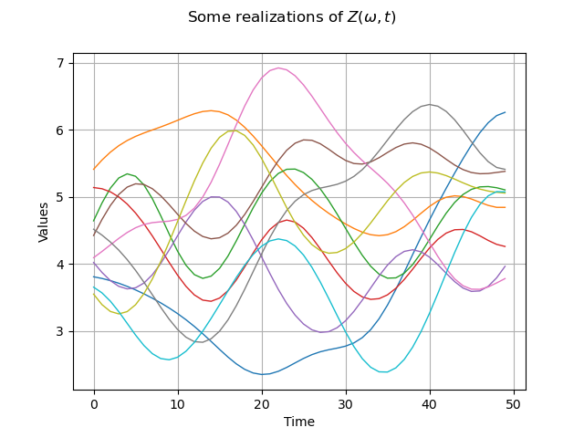
4. Draw some realizations of the process
N = 10
sampleZ_proc = Z_proc.getSample(N)
graph = sampleZ_proc.drawMarginal(0)
graph.setTitle(r"Some realizations of $Z(\omega, t)$")
view = View(graph)
5. Evaluate the probability that  
We define the domain ![\mathcal{D} = [2,4]](data:image/svg+xml;base64,PD94bWwgdmVyc2lvbj0nMS4wJyBlbmNvZGluZz0nVVRGLTgnPz4KPCEtLSBUaGlzIGZpbGUgd2FzIGdlbmVyYXRlZCBieSBkdmlzdmdtIDMuNC4yIC0tPgo8c3ZnIHZlcnNpb249JzEuMScgeG1sbnM9J2h0dHA6Ly93d3cudzMub3JnLzIwMDAvc3ZnJyB4bWxuczp4bGluaz0naHR0cDovL3d3dy53My5vcmcvMTk5OS94bGluaycgd2lkdGg9JzQ4Ljc1NDAwMXB0JyBoZWlnaHQ9JzExLjk1NTE2OHB0JyB2aWV3Qm94PScwIC04Ljk2NjM3NiA0OC43NTQwMDEgMTEuOTU1MTY4Jz4KPGRlZnM+CjxwYXRoIGlkPSdnMS01OScgZD0nTTIuMzMxMjU4IC4wNDc4MjFDMi4zMzEyNTgtLjY0NTU3OSAyLjEwNDExLTEuMTU5NjUxIDEuNjEzOTQ4LTEuMTU5NjUxQzEuMjMxMzgyLTEuMTU5NjUxIDEuMDQwMS0uODQ4ODE3IDEuMDQwMS0uNTg1ODAzUzEuMjE5NDI3IDAgMS42MjU5MDMgMEMxLjc4MTMyIDAgMS45MTI4MjctLjA0NzgyMSAyLjAyMDQyMy0uMTU1NDE3QzIuMDQ0MzM0LS4xNzkzMjggMi4wNTYyODktLjE3OTMyOCAyLjA2ODI0NC0uMTc5MzI4QzIuMDkyMTU0LS4xNzkzMjggMi4wOTIxNTQtLjAxMTk1NSAyLjA5MjE1NCAuMDQ3ODIxQzIuMDkyMTU0IC40NDIzNDEgMi4wMjA0MjMgMS4yMTk0MjcgMS4zMjcwMjQgMS45OTY1MTNDMS4xOTU1MTcgMi4xMzk5NzUgMS4xOTU1MTcgMi4xNjM4ODUgMS4xOTU1MTcgMi4xODc3OTZDMS4xOTU1MTcgMi4yNDc1NzIgMS4yNTUyOTMgMi4zMDczNDcgMS4zMTUwNjggMi4zMDczNDdDMS40MTA3MSAyLjMwNzM0NyAyLjMzMTI1OCAxLjQyMjY2NSAyLjMzMTI1OCAuMDQ3ODIxWicvPgo8cGF0aCBpZD0nZzItNTAnIGQ9J001LjI2MDI3NC0yLjAwODQ2OEg0Ljk5NzI2QzQuOTYxMzk1LTEuODA1MjMgNC44NjU3NTMtMS4xNDc2OTYgNC43NDYyMDItLjk1NjQxM0M0LjY2MjUxNi0uODQ4ODE3IDMuOTgxMDcxLS44NDg4MTcgMy42MjI0MTYtLjg0ODgxN0gxLjQxMDcxQzEuNzMzNDk5LTEuMTIzNzg2IDIuNDYyNzY1LTEuODg4OTE3IDIuNzczNTk5LTIuMTc1ODQxQzQuNTkwNzg1LTMuODQ5NTY0IDUuMjYwMjc0LTQuNDcxMjMzIDUuMjYwMjc0LTUuNjU0Nzk1QzUuMjYwMjc0LTcuMDI5NjM5IDQuMTcyMzU0LTcuOTUwMTg3IDIuNzg1NTU0LTcuOTUwMTg3Uy41ODU4MDMtNi43NjY2MjUgLjU4NTgwMy01LjczODQ4MUMuNTg1ODAzLTUuMTI4NzY3IDEuMTExODMxLTUuMTI4NzY3IDEuMTQ3Njk2LTUuMTI4NzY3QzEuMzk4NzU1LTUuMTI4NzY3IDEuNzA5NTg5LTUuMzA4MDk1IDEuNzA5NTg5LTUuNjkwNjZDMS43MDk1ODktNi4wMjU0MDUgMS40ODI0NDEtNi4yNTI1NTMgMS4xNDc2OTYtNi4yNTI1NTNDMS4wNDAxLTYuMjUyNTUzIDEuMDE2MTg5LTYuMjUyNTUzIC45ODAzMjQtNi4yNDA1OThDMS4yMDc0NzItNy4wNTM1NDkgMS44NTMwNTEtNy42MDM0ODcgMi42MzAxMzctNy42MDM0ODdDMy42NDYzMjYtNy42MDM0ODcgNC4yNjc5OTUtNi43NTQ2NyA0LjI2Nzk5NS01LjY1NDc5NUM0LjI2Nzk5NS00LjYzODYwNSAzLjY4MjE5Mi0zLjc1MzkyMyAzLjAwMDc0Ny0yLjk4ODc5MkwuNTg1ODAzLS4yODY5MjRWMEg0Ljk0OTQ0TDUuMjYwMjc0LTIuMDA4NDY4WicvPgo8cGF0aCBpZD0nZzItNTInIGQ9J000LjMxNTgxNi03Ljc4MjgxNEM0LjMxNTgxNi04LjAwOTk2MyA0LjMxNTgxNi04LjA2OTczOCA0LjE0ODQ0My04LjA2OTczOEM0LjA1MjgwMi04LjA2OTczOCA0LjAxNjkzNi04LjA2OTczOCAzLjkyMTI5NS03LjkyNjI3NkwuMzIyNzktMi4zNDMyMTNWLTEuOTk2NTEzSDMuNDY2OTk5Vi0uOTA4NTkzQzMuNDY2OTk5LS40NjYyNTIgMy40NDMwODgtLjM0NjcgMi41NzAzNjEtLjM0NjdIMi4zMzEyNThWMEMyLjYwNjIyNy0uMDIzOTEgMy41NTA2ODUtLjAyMzkxIDMuODg1NDMtLjAyMzkxUzUuMTc2NTg4LS4wMjM5MSA1LjQ1MTU1NyAwVi0uMzQ2N0g1LjIxMjQ1M0M0LjM1MTY4MS0uMzQ2NyA0LjMxNTgxNi0uNDY2MjUyIDQuMzE1ODE2LS45MDg1OTNWLTEuOTk2NTEzSDUuNTIzMjg4Vi0yLjM0MzIxM0g0LjMxNTgxNlYtNy43ODI4MTRaTTMuNTI2Nzc1LTYuODUwMzExVi0yLjM0MzIxM0guNjIxNjY5TDMuNTI2Nzc1LTYuODUwMzExWicvPgo8cGF0aCBpZD0nZzItNjEnIGQ9J004LjA2OTczOC0zLjg3MzQ3NEM4LjIzNzExMS0zLjg3MzQ3NCA4LjQ1MjMwNC0zLjg3MzQ3NCA4LjQ1MjMwNC00LjA4ODY2N0M4LjQ1MjMwNC00LjMxNTgxNiA4LjI0OTA2Ni00LjMxNTgxNiA4LjA2OTczOC00LjMxNTgxNkgxLjAyODE0NEMuODYwNzcyLTQuMzE1ODE2IC42NDU1NzktNC4zMTU4MTYgLjY0NTU3OS00LjEwMDYyM0MuNjQ1NTc5LTMuODczNDc0IC44NDg4MTctMy44NzM0NzQgMS4wMjgxNDQtMy44NzM0NzRIOC4wNjk3MzhaTTguMDY5NzM4LTEuNjQ5ODEzQzguMjM3MTExLTEuNjQ5ODEzIDguNDUyMzA0LTEuNjQ5ODEzIDguNDUyMzA0LTEuODY1MDA2QzguNDUyMzA0LTIuMDkyMTU0IDguMjQ5MDY2LTIuMDkyMTU0IDguMDY5NzM4LTIuMDkyMTU0SDEuMDI4MTQ0Qy44NjA3NzItMi4wOTIxNTQgLjY0NTU3OS0yLjA5MjE1NCAuNjQ1NTc5LTEuODc2OTYxQy42NDU1NzktMS42NDk4MTMgLjg0ODgxNy0xLjY0OTgxMyAxLjAyODE0NC0xLjY0OTgxM0g4LjA2OTczOFonLz4KPHBhdGggaWQ9J2cyLTkxJyBkPSdNMi45ODg3OTIgMi45ODg3OTJWMi41NDY0NTFIMS44MjkxNDFWLTguNTI0MDM1SDIuOTg4NzkyVi04Ljk2NjM3NkgxLjM4NjhWMi45ODg3OTJIMi45ODg3OTJaJy8+CjxwYXRoIGlkPSdnMi05MycgZD0nTTEuODUzMDUxLTguOTY2Mzc2SC4yNTEwNTlWLTguNTI0MDM1SDEuNDEwNzFWMi41NDY0NTFILjI1MTA1OVYyLjk4ODc5MkgxLjg1MzA1MVYtOC45NjYzNzZaJy8+CjxwYXRoIGlkPSdnMC02OCcgZD0nTTIuNDM4ODU0IDBDNS4yMjQ0MDggMCA5LjE1NzY1OS0yLjEyODAyIDkuMTU3NjU5LTUuMzkxNzgxQzkuMTU3NjU5LTYuNDU1NzkxIDguNjU1NTQyLTcuMTI1MjggOC4wNjk3MzgtNy40OTU4OUM3LjA0MTU5NC04LjE2NTM4IDUuOTQxNzE5LTguMTY1MzggNC44MDU5NzgtOC4xNjUzOEMzLjc3NzgzMy04LjE2NTM4IDMuMDcyNDc4LTguMTY1MzggMi4wNjgyNDQtNy43MzQ5OTRDLjQ3ODIwNy03LjAyOTYzOSAuMjUxMDU5LTYuMDM3MzYgLjI1MTA1OS01Ljk0MTcxOUMuMjUxMDU5LTUuODY5OTg4IC4yOTg4NzktNS44NDYwNzcgLjM3MDYxLTUuODQ2MDc3Qy41NjE4OTMtNS44NDYwNzcgLjgzNjg2Mi02LjAxMzQ1IC45MzI1MDMtNi4wNzMyMjVDMS4xODM1NjItNi4yNDA1OTggMS4yMTk0MjctNi4zMTIzMjkgMS4yOTExNTgtNi41Mzk0NzdDMS40NTg1MzEtNy4wMTc2ODQgMS43OTMyNzUtNy40MzYxMTUgMy4yOTk2MjYtNy41MDc4NDZDMy4xMDgzNDQtNS4wMDkyMTUgMi40OTg2My0yLjcyNTc3OCAxLjY2MTc2OC0uNjMzNjI0QzEuMjE5NDI3LS40NzgyMDcgLjkzMjUwMy0uMjAzMjM4IC45MzI1MDMtLjA4MzY4NkMuOTMyNTAzLS4wMTE5NTUgLjk0NDQ1OCAwIDEuMjA3NDcyIDBIMi40Mzg4NTRaTTIuNDk4NjMtLjY1NzUzNEMzLjg2MTUxOS0zLjk5MzAyNiA0LjExMjU3OC02LjA3MzIyNSA0LjI3OTk1LTcuNTA3ODQ2QzUuMDgwOTQ2LTcuNTA3ODQ2IDguMTQxNDY5LTcuNTA3ODQ2IDguMTQxNDY5LTQuODc3NzA5QzguMTQxNDY5LTIuNTM0NDk2IDYuMDM3MzYtLjY1NzUzNCAzLjE0NDIwOS0uNjU3NTM0SDIuNDk4NjNaJy8+CjwvZGVmcz4KPGcgaWQ9J3BhZ2UxJz4KPHVzZSB4PScwJyB5PScwJyB4bGluazpocmVmPScjZzAtNjgnLz4KPHVzZSB4PScxMi44NzUwNTgnIHk9JzAnIHhsaW5rOmhyZWY9JyNnMi02MScvPgo8dXNlIHg9JzI1LjMwMDUzOScgeT0nMCcgeGxpbms6aHJlZj0nI2cyLTkxJy8+Cjx1c2UgeD0nMjguNTUyMicgeT0nMCcgeGxpbms6aHJlZj0nI2cyLTUwJy8+Cjx1c2UgeD0nMzQuNDA1MTkxJyB5PScwJyB4bGluazpocmVmPScjZzEtNTknLz4KPHVzZSB4PSczOS42NDkzNScgeT0nMCcgeGxpbms6aHJlZj0nI2cyLTUyJy8+Cjx1c2UgeD0nNDUuNTAyMzQnIHk9JzAnIHhsaW5rOmhyZWY9JyNnMi05MycvPgo8L2c+Cjwvc3ZnPgo8IS0tIERFUFRIPTQgLS0+) and the event :
and the event :
domain = ot.Interval([2], [4])
print("D = ", domain)
event = ot.ProcessEvent(Z_proc, domain)
D = [2, 4]
We use the Monte Carlo sampling to evaluate the probability:
MC_algo = ot.ProbabilitySimulationAlgorithm(event)
MC_algo.setMaximumOuterSampling(1000000)
MC_algo.setBlockSize(100)
MC_algo.setMaximumCoefficientOfVariation(0.01)
MC_algo.run()

result = MC_algo.getResult()

proba = result.getProbabilityEstimate()
print("Probability = ", proba)
variance = result.getVarianceEstimate()
print("Variance Estimate = ", variance)
IC90_low = proba - result.getConfidenceLength(0.90) / 2
IC90_upp = proba + result.getConfidenceLength(0.90) / 2
print("IC (90%) = [", IC90_low, ", ", IC90_upp, "]")
view.ShowAll()
Probability =  0.7544117647058823
Variance Estimate =  5.50381483777321e-05
IC (90%) = [ 0.7422089739566764 ,  0.7666145554550883 ]