Note
Go to the end to download the full example code.
Create a stationary covariance model
This use case illustrates how the user can define his own stationary covariance model thanks to the object UserDefinedStationaryCovarianceModel defined from:
a mesh
 of dimension
  defined by the vertices
  and the associated simplices,
a collection of covariance matrices stored in the object
CovarianceMatrixCollectionnoted where
where 
 for
for 
Then we build a stationary covariance function which is a piecewise constant function on  defined by:

where  is such that
  is the vertex of the nearest to
import openturns as ot
import openturns.viewer as viewer
from matplotlib import pylab as plt

ot.Log.Show(ot.Log.NONE)
We detail the example described in the documentation
Create the time grid
t0 = 0.0
dt = 0.5
N = int((20.0 - t0) / dt)
mesh = ot.RegularGrid(t0, dt, N)

# Create the covariance function


def gamma(tau):
    return 1.0 / (1.0 + tau * tau)


# Create the collection of :class:`~openturns.SquareMatrix`
coll = ot.SquareMatrixCollection()
for k in range(N):
    t = mesh.getValue(k)
    matrix = ot.SquareMatrix([[gamma(t)]])
    coll.add(matrix)
Create the covariance model
covmodel = ot.UserDefinedStationaryCovarianceModel(mesh, coll)

# One vertex of the mesh
tau = 1.5

# Get the covariance function computed at the vertex tau
covmodel(tau)
Graph of the spectral function
x = ot.Sample(N, 2)
for k in range(N):
t = mesh.getValue(k)
x[k, 0] = t
value = covmodel(t)
x[k, 1] = value[0, 0]
# Create the curve of the spectral function
curve = ot.Curve(x, "User Model")
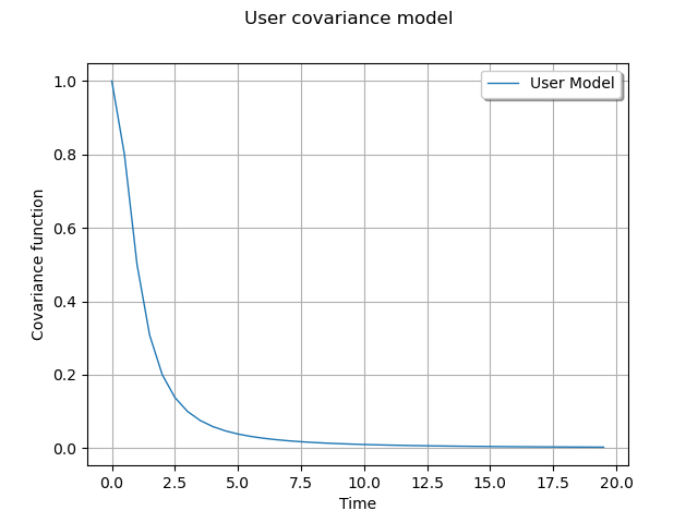
# Create the graph
myGraph = ot.Graph("User covariance model", "Time", "Covariance function", True)
myGraph.add(curve)
myGraph.setLegendPosition("upper right")
view = viewer.View(myGraph)
plt.show()