Analyse the central tendency of a cantilever beam

In this example we perform a central tendency analysis of a random variable Y using the various methods available. We consider the cantilever beam example and show how to use the TaylorExpansionMoments and ExpectationSimulationAlgorithm classes.

from openturns.usecases import cantilever_beam
import openturns as ot
import openturns.viewer as viewer
from matplotlib import pylab as plt

ot.Log.Show(ot.Log.NONE)

We first load the data class from the usecases module :

cb = cantilever_beam.CantileverBeam()

We want to create the random variable of interest where is the physical model and is the input vectors.

We create the input parameters distribution and make a random vector. For the sake of this example, we consider an independent copula.

distribution = ot.JointDistribution([cb.E, cb.F, cb.L, cb.II])
X = ot.RandomVector(distribution)
X.setDescription(["E", "F", "L", "I"])

f is the cantilever beam model :

f = cb.model

The random variable of interest Y is then

Y = ot.CompositeRandomVector(f, X)
Y.setDescription("Y")

Taylor expansion

Perform Taylor approximation to get the expected value of Y and the importance factors.

taylor = ot.TaylorExpansionMoments(Y)
taylor_mean_fo = taylor.getMeanFirstOrder()
taylor_mean_so = taylor.getMeanSecondOrder()
taylor_cov = taylor.getCovariance()
taylor_if = taylor.getImportanceFactors()
print("model evaluation calls number=", f.getGradientCallsNumber())
print("model gradient calls number=", f.getGradientCallsNumber())
print("model hessian calls number=", f.getHessianCallsNumber())
print("taylor mean first order=", taylor_mean_fo)
print("taylor variance=", taylor_cov)
print("taylor importance factors=", taylor_if)

model evaluation calls number= 1
model gradient calls number= 1
model hessian calls number= 1
taylor mean first order= [0.170111]
taylor variance= [[ 0.00041128 ]]
taylor importance factors= [E : 0.0471628, F : 0.703601, L : 0.0811537, I : 0.168082]

graph = taylor.drawImportanceFactors()
view = viewer.View(graph)

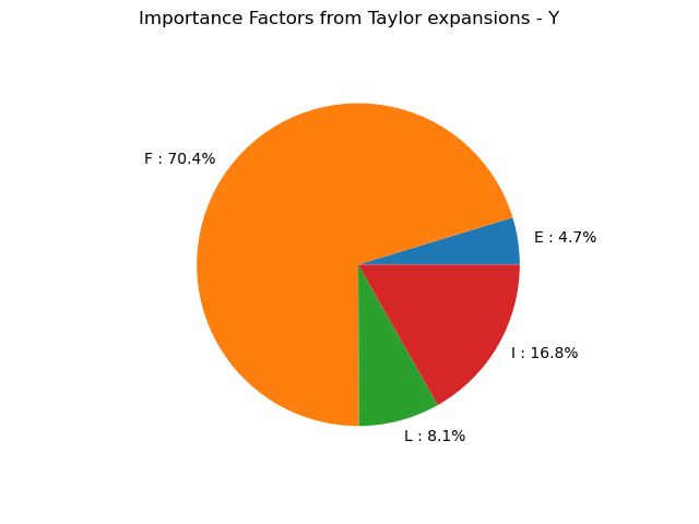
We see that, at first order, the variable explains about 70% of the variance of the output . On the other hand, the variable is the least significant in the variance of the output: only explains about 5% of the output variance.

Monte-Carlo simulation

Perform a Monte Carlo simulation of Y to estimate its mean.

algo = ot.ExpectationSimulationAlgorithm(Y)
algo.setMaximumOuterSampling(1000)
algo.setCoefficientOfVariationCriterionType("NONE")
algo.run()
print("model evaluation calls number=", f.getEvaluationCallsNumber())
expectation_result = algo.getResult()
expectation_mean = expectation_result.getExpectationEstimate()
print(
    "monte carlo mean=",
    expectation_mean,
    "var=",
    expectation_result.getVarianceEstimate(),
)

model evaluation calls number= 1001
monte carlo mean= [0.170358] var= [4.16495e-07]

Central dispersion analysis based on a sample

Directly compute statistical moments based on a sample of Y. Sometimes the probabilistic model is not available and the study needs to start from the data.

Y_s = Y.getSample(1000)
y_mean = Y_s.computeMean()
y_stddev = Y_s.computeStandardDeviation()
y_quantile_95p = Y_s.computeQuantilePerComponent(0.95)
print("mean=", y_mean, "stddev=", y_stddev, "quantile@95%", y_quantile_95p)

mean= [0.17029] stddev= [0.0206972] quantile@95% [0.206341]

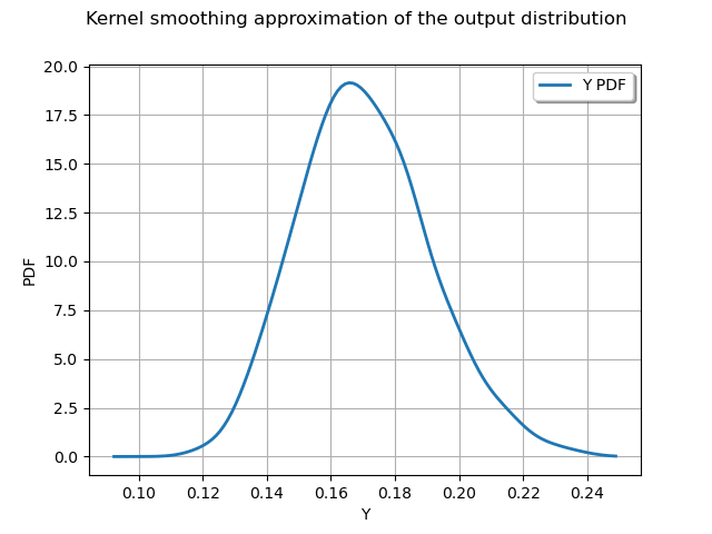
graph = ot.KernelSmoothing().build(Y_s).drawPDF()
graph.setTitle("Kernel smoothing approximation of the output distribution")
view = viewer.View(graph)

plt.show()