Plot the Smolyak quadrature

The goal of this example is to present different properties of Smolyak’s quadrature.

import openturns as ot
import openturns.viewer as otv
from matplotlib import pylab as plt

In the first example, we plot the nodes different levels of Smolyak-Legendre quadrature.

uniform = ot.GaussProductExperiment(ot.Uniform(-1.0, 1.0))
collection = [uniform] * 2

In the following loop, the level increases from 1 to 6. For each level, we create the associated Smolyak quadrature and plot the associated nodes.

number_of_rows = 2
number_of_columns = 3
bounding_box = ot.Interval([-1.05] * 2, [1.05] * 2)
grid = ot.GridLayout(number_of_rows, number_of_columns)
for i in range(number_of_rows):
    for j in range(number_of_columns):
        level = 1 + j + i * number_of_columns
        experiment = ot.SmolyakExperiment(collection, level)
        nodes, weights = experiment.generateWithWeights()
        sample_size = weights.getDimension()
        graph = ot.Graph(
            r"Level = %d, n = %d" % (level, sample_size), "$x_1$", "$x_2$", True
        )
        cloud = ot.Cloud(nodes)
        cloud.setPointStyle("circle")
        graph.add(cloud)
        graph.setBoundingBox(bounding_box)
        grid.setGraph(i, j, graph)

unit_width = 2.0
total_width = unit_width * number_of_columns
unit_height = unit_width
total_height = unit_height * number_of_rows
view = otv.View(grid, figure_kw={"figsize": (total_width, total_height)})
_ = plt.suptitle("Smolyak-Legendre")
_ = plt.subplots_adjust(wspace=0.4, hspace=0.4)
plt.tight_layout()
plt.show()

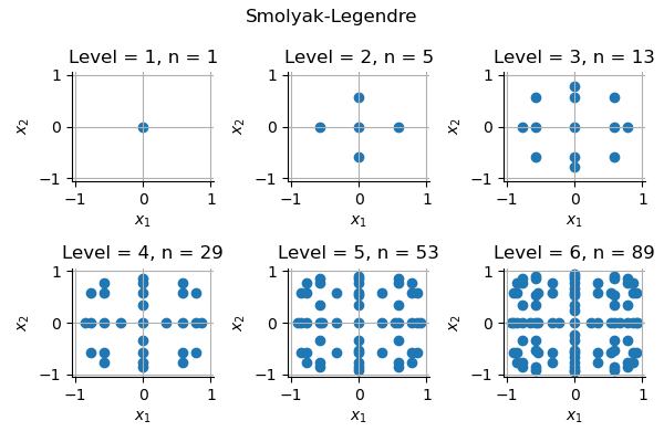
In the previous plot, the number of nodes is denoted by . We see that the number of nodes in the quadrature slowly increases when the quadrature level increases.

Secondly, we want to compute the number of nodes depending on the dimension and the level.

Assume that the number of nodes depends on the level from the equation . In a fully tensorized grid, the number of nodes is ([gerstner1998] page 216):

We are going to see that Smolyak’s quadrature reduces drastically that number. Let be the number of the marginal univariate quadrature of level . The number of nodes in Smolyak’s sparse grid is:

If , then the number of nodes of Smolyak’s quadrature is:

In the following script, we plot the number of nodes versus the level, of the tensor product and Smolyak experiments, under the assumption that and . In other words, we assume that the constants involved in the previous Landau equations are equal to 1.

level_max = 8  # Maximum level
dimension_max = 8  # Maximum dimension
level_list = list(range(1, 1 + level_max))
graph = ot.Graph(
    "Smolyak vs tensorized quadrature", r"$level$", r"$n$", True, "upper left"
)
dimension_list = list(range(1, dimension_max, 2))
palette = ot.Drawable().BuildDefaultPalette(len(dimension_list))
graph_index = 0
for dimension in dimension_list:
    number_of_nodes = ot.Sample(level_max, 1)
    # Tensorized
    for level in level_list:
        number_of_nodes[level - 1, 0] = 2 ** (level * dimension)
    curve = ot.Curve(ot.Sample.BuildFromPoint(level_list), number_of_nodes)
    curve.setLegend("")
    curve.setLineStyle("solid")
    curve.setColor(palette[graph_index])
    curve.setLegend("Tensor, d = %d" % (dimension))
    graph.add(curve)
    # Smolyak
    for level in level_list:
        number_of_nodes[level - 1, 0] = 2**level * level ** (dimension - 1)
    curve = ot.Curve(ot.Sample.BuildFromPoint(level_list), number_of_nodes)
    curve.setLegend("")
    curve.setLineStyle("dashed")
    curve.setColor(palette[graph_index])
    curve.setLegend("Smolyak, d = %d" % (dimension))
    graph.add(curve)
    graph_index += 1
graph.setLogScale(ot.GraphImplementation.LOGY)
graph.setLegendCorner([1.0, 1.0])
graph.setLegendPosition("upper left")
view = otv.View(
    graph,
    figure_kw={"figsize": (5.0, 3.0)},
)
plt.tight_layout()
plt.show()

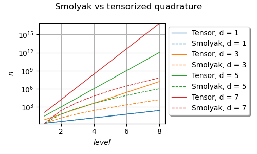
We see that the number of nodes increases when the level increases. Smolyak’s number of nodes is, however, smaller or equal to the number of nodes involved in a tensor product quadrature rule. In dimension 7 for example, the quadrature level 8 leads to less than nodes with Smolyak’s quadrature but more than nodes with a tensor product quadrature.

In the following cell, we count the number of nodes in Smolyak’s quadrature using a Gauss-Legendre marginal univariate experiment. We perform a loop over the levels from 1 to 8 and the dimensions from 1 to 7.

level_max = 8  # Maximum level
dimension_max = 8  # Maximum dimension
uniform = ot.GaussProductExperiment(ot.Uniform(-1.0, 1.0))
level_list = list(range(1, 1 + level_max))
graph = ot.Graph("Smolyak-Legendre quadrature", r"$level$", r"$n$", True, "upper left")
palette = ot.Drawable().BuildDefaultPalette(dimension_max - 1)
graph_index = 0
for dimension in range(1, dimension_max):
    number_of_nodes = ot.Sample(level_max, 1)
    for level in level_list:
        collection = [uniform] * dimension
        experiment = ot.SmolyakExperiment(collection, level)
        nodes, weights = experiment.generateWithWeights()
        size = nodes.getSize()
        number_of_nodes[level - 1, 0] = size
    cloud = ot.Cloud(ot.Sample.BuildFromPoint(level_list), number_of_nodes)
    cloud.setLegend("$d = %d$" % (dimension))
    cloud.setPointStyle("bullet")
    cloud.setColor(palette[graph_index])
    graph.add(cloud)
    curve = ot.Curve(ot.Sample.BuildFromPoint(level_list), number_of_nodes)
    curve.setLegend("")
    curve.setLineStyle("dashed")
    curve.setColor(palette[graph_index])
    graph.add(curve)
    graph_index += 1
graph.setLogScale(ot.GraphImplementation.LOGY)
graph.setLegendCorner([1.0, 1.0])
graph.setLegendPosition("upper left")
view = otv.View(
    graph,
    figure_kw={"figsize": (5.0, 3.0)},
)

plt.tight_layout()
plt.show()

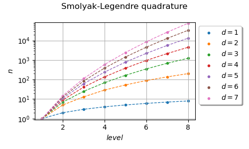
We see that the number of nodes increases when the level increases. This growth depends on the dimension of the problem.