Validation and cross validation of metamodels
Introduction
In ordinary validation of a metamodel, we hold some observations from the sample and train the model on the remaining observations. Then, we test the metamodel against the hold out observations. One of the problems of this method is that the surrogate model is trained using only a subset of the available data. As a consequence, the estimated error can be pessimistic or, on the contrary, overly optimistic. In cross-validation, the entirety of the data set is sequentially used for either training or validation. Hence, more of the available data is used, resulting in an improved accuracy of the estimated error of the metamodel. One of the problems of cross-validation is that we have to train the metamodel several times, which can be time consuming. In this case, the fast methods that we present below can be useful.
Let  be a physical
model where
be a physical
model where  is the domain of the input parameters
  .
Let
.
Let  be a metamodel of
  , i.e.
an approximation of the function.
Once the metamodel
of the original numerical model has been
built, we may estimate the mean squared error, i.e. the
discrepancy between the response surface and the true model response
in terms of the weighted
, i.e.
an approximation of the function.
Once the metamodel
of the original numerical model has been
built, we may estimate the mean squared error, i.e. the
discrepancy between the response surface and the true model response
in terms of the weighted  -norm:

where  is the probability density function
of the random vector
is the probability density function
of the random vector  .
In this section, we present the cross-validation of linear least squares
models, as presented in [wang2012] page 485.
.
In this section, we present the cross-validation of linear least squares
models, as presented in [wang2012] page 485.
The fraction of variance unexplained (FVU) is:

where  is the variance of the random output
  .
The fraction of variance unexplained is a relative mean squared error.
The coefficient of determination is:
.
The fraction of variance unexplained is a relative mean squared error.
The coefficient of determination is:

Simple validation
In the ordinary or naive validation method, we divide the data sample (i.e.
the experimental design) into two independent sub-samples:
the training and the test set.
In this case, the metamodel
is built from one sub-sample, i.e. the training set, and its
performance is assessed by comparing its predictions to the other
subset, i.e. the test set.
A single split will lead to a validation estimate.
When several splits are created, the cross-validation error
estimate is obtained by averaging over the splits.
When the coefficient of determination is evaluated on a test set which is
independent from the training set, the coefficient of determination is
sometimes called the  score.
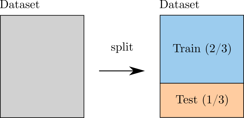
Figure 1. Validation using one single split.
Let  be an integer representing the sample size.
Let
be an integer representing the sample size.
Let  be a set of
  independent
observations of the random vector :
independent
observations of the random vector :

and consider the corresponding outputs of the model:

where:

for  .
The Monte-Carlo estimator of the mean squared error is:
.
The Monte-Carlo estimator of the mean squared error is:

The previous equation can be equivalently expressed depending on
the model since  .
It seems, however, more consistent to use
.
It seems, however, more consistent to use  because the
true model is unknown (otherwise we would not use a
surrogate).
because the
true model is unknown (otherwise we would not use a
surrogate).
The sample relative mean squared error is:

where  is the sample variance of the random output:

where  is the sample mean of the output:

If the test set  is not independent from the training set
(the set used to calibrate the metamodel), then the previous estimator
may underestimate the true value of the mean squared error.
Assuming that the sample is made of i.i.d. observations,
in order to create a test set independent from the training set, a
simple method is to split the data set into two parts.
The drawback of this method is that this reduces the size of the training
set, so that the mean squared error evaluated on the test set can be pessimistic
(because the metamodel is trained with less data) or optimistic (because the R2
score has a greater variability).
The leave-one-out (LOO) and K-Fold cross validation methods presented in the next sections
have the advantage of using all of the available data.
is not independent from the training set
(the set used to calibrate the metamodel), then the previous estimator
may underestimate the true value of the mean squared error.
Assuming that the sample is made of i.i.d. observations,
in order to create a test set independent from the training set, a
simple method is to split the data set into two parts.
The drawback of this method is that this reduces the size of the training
set, so that the mean squared error evaluated on the test set can be pessimistic
(because the metamodel is trained with less data) or optimistic (because the R2
score has a greater variability).
The leave-one-out (LOO) and K-Fold cross validation methods presented in the next sections
have the advantage of using all of the available data.
Naive and fast cross-validation
As seen in the previous section, the simplest method of performing the validation consists in splitting the data into a training set and a test set. Moreover, provided these two sets are independent, then the estimate of the error is unbiased. In order to use all the available data instead of a subset of it, two other estimators can be considered: the leave-one-out and K-Fold estimators, which are the topic of the next sections.
When implemented naively, these methods may require to build many metamodels, which can be time-consuming. Fortunately, there are shortcuts for many metamodels including linear least squares and splines (and others). For a linear least squares model, some methods use the Sherman-Morrisson-Woodbury formula to get updates of the inverse Gram matrix, as we are going to see later in this document. This makes it possible to easily evaluate metamodel errors of a linear least squares model.
Leave-one-out cross-validation
In this section, we present the naive leave-one-out error estimator,
also known as jackknife in statistics.
Let  be the metamodel estimated from the
leave-one-out experimental design
be the metamodel estimated from the
leave-one-out experimental design  .
This is the experimental design where the
.
This is the experimental design where the  -th observation
 is set aside.
The corresponding set of observation indices is:
is set aside.
The corresponding set of observation indices is:

the corresponding input observations are:

and the corresponding output observations are:

The leave-one-out residual is defined as the difference between the model evaluation at
and its leave-one-out prediction (see [blatman2009]
eq. 4.26 page 85):

We repeat this process for all observations in the experimental
design and obtain the predicted residuals
 for
for  .
Finally, the LOO mean squared error estimator is:
.
Finally, the LOO mean squared error estimator is:

One of the drawbacks of the naive method is that it may require
to estimate different metamodels.
If is large or if training each metamodel is costly,
then the leave-one-out method can be impractical.
If, however, the metamodel is based on the linear least squares method,
then the leave-one-out error may be computed much more efficiently, as
shown in the next section.
Fast leave-one-out cross-validation of a linear model
In this section, we present the fast leave-one-out error estimator
of a linear least squares model.
In the special case of a linear least squares model, [stone1974] (see eq. 3.13 page 121)
showed that the leave-one-out residuals have an expression which depends on the diagonal
of the projection matrix.
In this case, the evaluation of the leave-one-out mean squared error involves the
multiplication of the raw residuals by a correction which involves the leverages
of the model.
This method makes it possible to directly evaluate the mean squared error without
necessarily estimating the coefficients of different leave-one-out
least squares models.
It is then much faster than the naive leave-one-out method.
Assume that the model is linear:

for any  where
where  is the vector of parameters.
Let
is the vector of parameters.
Let  be the vector of output observations:

The goal of the least squares method is to estimate the coefficients
 using the vector of observations
  .
The output vector from the linear model is:
.
The output vector from the linear model is:

for any where
 is the
design matrix.
For a linear model, the columns of the design matrix correspond
to the input parameters and the rows correspond to the observations:
is the
design matrix.
For a linear model, the columns of the design matrix correspond
to the input parameters and the rows correspond to the observations:

In the previous equation, notice that the design matrix depends on the
experimental design .
Assume that the matrix  has full rank.
The solution of the linear least squares problem is
given by the normal equations (see [Bjorck1996] eq. 1.1.15 page 6):
has full rank.
The solution of the linear least squares problem is
given by the normal equations (see [Bjorck1996] eq. 1.1.15 page 6):

The linear metamodel is the linear model with estimated coefficients:

The vector of predictions from the metamodel is:

for any where  is the
estimate from linear least squares.
We substitute the estimator in the previous equation and
get the value of the surrogate linear model:
is the
estimate from linear least squares.
We substitute the estimator in the previous equation and
get the value of the surrogate linear model:

Let  be the projection (“hat”) matrix (see [wang2012] eq. 16.8 page 472):

Hence, the value of the linear model is the matrix-vector product:

We can prove that the LOO residual is:
(1)
where  is the -th diagonal term of the hat matrix.
In other words, the residual of the LOO metamodel is equal to the
residual of the full metamodel corrected by
is the -th diagonal term of the hat matrix.
In other words, the residual of the LOO metamodel is equal to the
residual of the full metamodel corrected by  .
.
The number is the leverage of the -th
observation.
It can be proved (see [sen1990] page 157) that:

Moreover (see [sen1990] eq. 5.10 page 106):

where  is the trace of the hat matrix.
The leverage describes how far away the individual data point is from the centroid
of all data points (see [sen1990] page 155).
The equation (1) implies that if is
large (i.e. close to 1), then removing the -th observation
from the training sample changes the residual of the leave-one-out
metamodel significantly.
is the trace of the hat matrix.
The leverage describes how far away the individual data point is from the centroid
of all data points (see [sen1990] page 155).
The equation (1) implies that if is
large (i.e. close to 1), then removing the -th observation
from the training sample changes the residual of the leave-one-out
metamodel significantly.
Using the equation (1) avoids to actually build the LOO surrogate. We substitute the previous expression in the definition of the leave-one-out mean squared error estimator and get the fast leave-one-out cross validation error (see [wang2012] eq. 16.25 page 487):

Corrected leave-one-out
A penalized variant of the leave-one-out mean squared error may be used in order to increase its robustness with respect to overfitting. This is done using a criterion which takes into account the number of coefficients compared to the size of the experimental design. The corrected leave-one-out error is (see [chapelle2002], [blatman2009] eq. 4.38 page 86):

where the penalty factor is:

where  is the matrix:

and  is the trace operator.
K-fold cross-validation
In this section, we present the naive K-Fold cross-validation.
Let  be a parameter representing the number of
splits in the data set.
The
be a parameter representing the number of
splits in the data set.
The  -fold cross-validation technique relies on splitting the
data set into sub-samples
-fold cross-validation technique relies on splitting the
data set into sub-samples
 , called the folds.
The corresponding set of indices:
, called the folds.
The corresponding set of indices:

and the corresponding set of input observations is:

The next figure presents this type of cross validation.

Figure 2. K-Fold cross-validation.
The folds are generally chosen to be of
approximately equal sizes.
If the sample size is a multiple of , then the
folds can have exactly the same size.
For any  , let
, let  be the metamodel estimated on the K-fold sample
 .
Let
.
Let  be defined as the K-Fold residual:

for  and
and  .
In the previous equation, the predicted residual
.
In the previous equation, the predicted residual
 is the difference between the
evaluation of and the value of the K-Fold surrogate
at the point .
The local approximation error is estimated on the sample
is the difference between the
evaluation of and the value of the K-Fold surrogate
at the point .
The local approximation error is estimated on the sample  :
:

where  is the number of observations in
the sub-sample :
is the number of observations in
the sub-sample :

For any  , the K-Fold mean square error
  is estimated using
the training set and
the test set .
Finally, the global K-fold cross-validation error estimate is the
sample mean (see [burman1989] page 505):
is estimated using
the training set and
the test set .
Finally, the global K-fold cross-validation error estimate is the
sample mean (see [burman1989] page 505):
(2)
The weight  reflects the fact that a fold containing
more observations weighs more in the estimator.
The K-Fold error estimate can be obtained
with a single split of the data into folds.
The leave-one-out (LOO) cross-validation is a special case of
the K-Fold cross-validation where the number of folds is
equal to , the sample size of the experimental design
.
reflects the fact that a fold containing
more observations weighs more in the estimator.
The K-Fold error estimate can be obtained
with a single split of the data into folds.
The leave-one-out (LOO) cross-validation is a special case of
the K-Fold cross-validation where the number of folds is
equal to , the sample size of the experimental design
.
We substitute the previous equation in the definition of the K-Fold MSE and get:

This implies:

The previous equation states that the K-Fold mean squared error is the sample mean of the corrected K-Fold squared residuals.
Assume that the number of folds divides the sample size.
Mathematically, this means that divides .
In this special case, each fold has the same number of observations:

for . Hence all local K-Fold MSE have the
same weight and we have  for .
This implies that the K-Fold mean squared error has a particularly simple expression
(see [deisenroth2020] eq. 8.13 page 264):
for .
This implies that the K-Fold mean squared error has a particularly simple expression
(see [deisenroth2020] eq. 8.13 page 264):
(3)
Fast K-Fold cross-validation of a linear model
In this section, we present a fast version of the K-Fold cross-validation
that can be used for a linear model.
While evaluating the mean squared error with the fast LOO formula involves the division by ,
using the fast K-Fold method involves the resolution of a linear system of
equations (see [shao1993] and [suzuki2020] proposition 14 page 71).
For any , let  be the rows of the design matrix corresponding to the indices of the observations
involved in the
be the rows of the design matrix corresponding to the indices of the observations
involved in the  -th fold:

where  are the
indices of the observations involved in the -th fold.
For any ,
let
are the
indices of the observations involved in the -th fold.
For any ,
let  be the sub-matrix of
the hat matrix corresponding to the indices of the observations in the
-th fold:
be the sub-matrix of
the hat matrix corresponding to the indices of the observations in the
-th fold:

It is not necessary to evaluate the previous expression in order to evaluate
the corresponding hat matrix.
Indeed, the matrix  can be computed by extracting the corresponding
rows and columns from the full hat matrix
can be computed by extracting the corresponding
rows and columns from the full hat matrix  :
:

Let  be the vector of
corrected K-Fold residuals:
be the vector of
corrected K-Fold residuals:

where  is the identity matrix,
 is the vector of output observations in the
-th fold:
is the vector of output observations in the
-th fold:

and  is the corresponding
vector of output predictions from the linear least squares metamodel:
is the corresponding
vector of output predictions from the linear least squares metamodel:

Then the mean squared error of the -th fold is:

Then the K-Fold mean squared error is evaluated from equation (2).
Cross-validation and model selection
If a model selection method is used (such as LARS), then the fast cross-validation (CV)
method can produce an optimistic estimated error, i.e. the true error can
be greater than the estimated error (see [hastie2009] section 7.10.2 page 245).
This is because the fast CV does not take model selection into account.
The reason for this behavior is that the model selection produces a set of predictors which fits the data particularly well. If a model selection method is involved, only the simple validation method can produce an unbiased estimator, because the model selection is then involved each time a new metamodel is trained i.e. each time its coefficients are estimated. The fast method, on the other hand, only considers the basis which is the result of a single training step.
Notice, however, that the order of magnitude of the error estimated using the fast method with a metamodel involving a model selection may be satisfactory in some cases.
Conclusion
The generic cross-validation method can be implemented using the following classes:
MetaModelValidation: uses a test set to compute the mean squared error ;LeaveOneOutSplitter: uses the leave-one-out method to split the data set ;KFoldSplitter: uses the K-Fold method to split the data set.
Since LinearModelResult is based on linear least
squares, fast methods are implemented in LinearModelValidation.