User manual
In the context of sensitivity analysis, we often have to deal with high dimensional inputs and heavy CPU time codes. Thus usual sensitivity techniques based on ANOVA reach their limits as they require to discretize conditional variance, which needs several samples to get an accurate approximation.
To tackle this kind of problems, screening methods could be applied in order to get a qualitative sensitivity estimate. The Morris method address the needs.
The method focuses on the notion of elementary effects and is known to require very few simulations to get an accurate estimate of the influent factors.
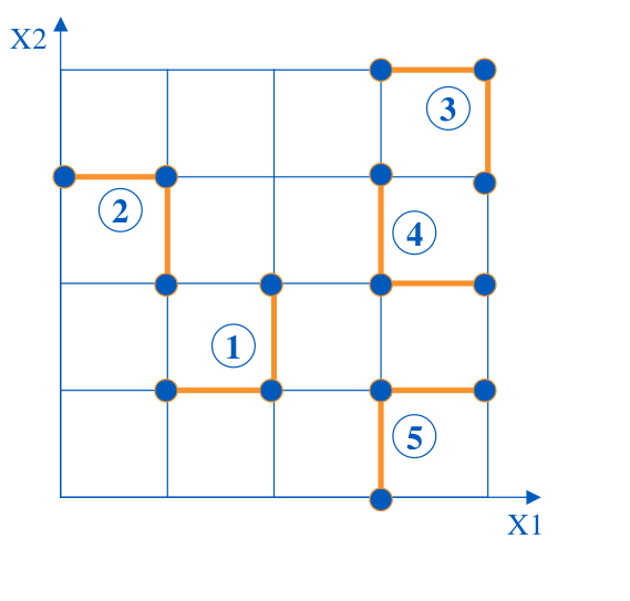
Roughly speeking, the method relies on One At Time designs (OAT) and acts as follows:
The input design space is discretized (in a p-levels grid), of step
 ;
;We randomly choose a starting point in this grid;
We randomly select a direction and thus we get the new point,
We iterate the previous process on the
 remaining directions to get a full path, where
  is the input dimension.
Note that
is the input dimension.
Note that  experiments are needed to define this path. (See hereafter an example in case
  )
)
From this path (
 ), we compute the response answer
  ;
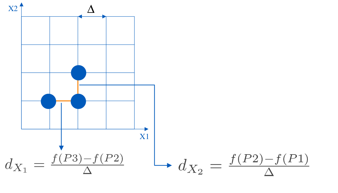
;It is easy to see that the difference between two consecutive points of this path represents the elementary effect relative to the chosen direction. Indeed we compute both
 and
and  where represents the difference between
two consecutive elements of .
We deduce elementary effects from these vectors of size by solving the linear system
where represents the difference between
two consecutive elements of .
We deduce elementary effects from these vectors of size by solving the linear system
 (
( are the elementary effects)
We iterate the steps 2-5
 times in order to get r replicates of the elementary effects.
Here after an illustration in case
times in order to get r replicates of the elementary effects.
Here after an illustration in case  .
.
If we note  the k-th computed elementary effects associated to the i-th input marginal,
it follows that from the r-sample of elementary effects,
we get
the k-th computed elementary effects associated to the i-th input marginal,
it follows that from the r-sample of elementary effects,
we get  respectively the absolute mean and the standard deviation of the elementary effects:

These are the measure used to get a qualitative approch of the sensitivity.
In the original Morris implementation, the mean of elementary effects  was used but it lacks of precision due to some potential sign changes. The previous values could be interpreted as follows:
 measures sensitivity. Important values highlight important effects and thus that model is sensitive to input variations,
 measures the interactions and non linearity effects.
Important values could explains non linear effects or interactions but it is impossible to make the distinction between the two cases.
measures the interactions and non linearity effects.
Important values could explains non linear effects or interactions but it is impossible to make the distinction between the two cases.
In engineering application literature, other interpretations could be found based on the quantity  :
:
If
 the i-th variable has almost linear effects,
If
 the i-th variable has monotonic effects,
If
 the i-th variable has quasi-monotonic effects,
If
 the i-th variable has non-linear and non-monotonic effects
To conclude, this module allows one to estimate the previous sensitivity measures (both  )
starting both from a p-level grid or an LHS experiment.
It allows also to get response model outside the library and finally plot the sensitivity to get a qualitative estimate.
)
starting both from a p-level grid or an LHS experiment.
It allows also to get response model outside the library and finally plot the sensitivity to get a qualitative estimate.
Reference
Campolongo, F., S. Tarantola and A. Saltelli. (1999). “Tackling quantitatively large dimensionality problems.”. Computer Physics Communication 1999: 75–85. pdf
Morris, M.D. (1991). “Factorial Sampling Plans for Preliminary Computational Experiments” (PDF). Technometrics 33: 161–174. pdf
Campolongo, Cariboni, Saltelli, F., J.and A. (2003). “Sensitivity analysis: the Morris method versus the variance based measures. Submitted to Technometrics” (PDF).
Andrea Saltelli, Stefano Tarantola,Francesca Campolongo and Marco Ratto (2004). “Sensitivity analysis in practice a guide to assessing scientific models”. John Willy & sons pdf
Experiments for Morris
|
Base class for the Morris method experiments. |
|
MorrisExperimentGrid builds experiments for the Morris method starting from full p-levels grid experiments. |
|
MorrisExperimentLHS builds experiments for the Morris method using a centered LHS design as input starting. |
Morris screening method
|
Morris method. |
Morris function
|
Morris test function for sensitivity analysis. |