Viscous free fall: metamodel of a field function¶

In this example, we present how to create the metamodel of a field function. This examples considers the free fall model. We first compute the Karhunen-Loève decomposition of a sample of trajectories. Then we create a create a polynomial chaos which takes the inputs and returns the KL decomposition modes as outputs. Finally, we create a metamodel by combining the KL decomposition and the polynomial chaos.

Introduction¶

We consider an object inside a vertical cylinder which contains a viscous fluid. The fluid generates a drag force which limits the speed of the solid and we assume that the force depends linearily on the object speed:

$m \frac{dv}{dt} = - m g - c v$

for any $t \in [0, t_{max}]$ where:

$v$ is the speed $[m/s]$ ,
$t$ is the time $[s]$ ,
$t_{max}$ is the maximum time $[s]$ ,
$g$ is the gravitational acceleration $[m.s^{-2}]$ ,
$m$ is the mass $[kg]$ ,
$c$ is the linear drag coefficient $[kg.s^{-1}]$ .

The previous differential equation has the exact solution:

$z(t) = z_0 + v_{inf} t + \tau (v_0 - v_{inf})\left(1 - e^{-\frac{t}{\tau}}\right)$

for any $t \in [0, t_{max}]$

where:

$z$ is the altitude above the surface $[m]$ ,
$z_0$ is the initial altitude $[m]$ ,
$v_0$ is the initial speed (upward) $[m.s^{-1}]$ ,
$v_{inf}$ is the limit speed $[m.s^{-1}]$ :

$v_{inf}=-\frac{m g}{c}$

$\tau$ is time caracteristic $[s]$ :

$\tau=\frac{m}{c}.$

The stationnary speed limit at infinite time is equal to $v_{inf}$ :

$\lim_{t\rightarrow+\infty} v(t)= v_{inf}.$

When there is no drag, i.e. when $c=0$ , the trajectory depends quadratically on $t$ :

$z(t) = z_0 + v_0 t -g t^2$

for any $t \in [0, t_{max}]$ .

Furthermore, when the solid touches the ground, we ensure that the altitude remains nonnegative, i.e. the final altitude is:

$y(t) = \max(z(t),0)$

for any $t \in [0, t_{max}]$ .

Probabilistic model¶

The parameters $z_0$ , $v_0$ , $m$ and $c$ are probabilistic:

$z_0 \sim \mathcal{U}(100, 150)$ ,
$v_0 \sim \mathcal{N}(55, 10)$ ,
$m \sim \mathcal{N}(80, 8)$ ,
$c \sim \mathcal{U}(0, 30)$ .

References¶

Steven C. Chapra. Applied numerical methods with Matlab for engineers and scientists, Third edition. 2012. Chapter 7, “Optimization”, p.182.

Define the model¶

[1]:

from __future__ import print_function
import openturns as ot
import numpy as np

We first define the time grid associated with the model.

[2]:

tmin=0.0 # Minimum time
tmax=12. # Maximum time
gridsize=100 # Number of time steps
mesh = ot.IntervalMesher([gridsize-1]).build(ot.Interval(tmin, tmax))

[3]:

vertices = mesh.getVertices()

Creation of the input distribution.

[4]:

distZ0 = ot.Uniform(100.0, 150.0)
distV0 = ot.Normal(55.0, 10.0)
distM = ot.Normal(80.0, 8.0)
distC = ot.Uniform(0.0, 30.0)
distribution = ot.ComposedDistribution([distZ0, distV0, distM, distC])

[5]:

dimension = distribution.getDimension()
dimension

[5]:

Then we define the Python function which computes the altitude at each time value. In order to compute all altitudes with a vectorized evaluation, we first convert the vertices into a Numpy array and use the Numpy functionsexp and maximum: this increases the evaluation performance of the script.

[6]:

def AltiFunc(X):
    g  = 9.81
    z0 = X[0]
    v0 = X[1]
    m  = X[2]
    c  = X[3]
    tau = m / c
    vinf = - m * g / c
    t = np.array(vertices)
    z = z0 + vinf * t + tau * (v0 - vinf) * (1 - np.exp( - t / tau))
    z = np.maximum(z,0.)
    return [[zeta[0]] for zeta in z]

In order to create a Function from this Python function, we use the PythonPointToFieldFunction class. Since the altitude is the only output field, the third argument outputDimension is equal to 1. If we had computed the speed as an extra output field, we would have set 2 instead.

[7]:

outputDimension = 1
alti = ot.PythonPointToFieldFunction(dimension, mesh, outputDimension, AltiFunc)

Compute a training sample.

[8]:

size = 2000
ot.RandomGenerator.SetSeed(0)
inputSample = distribution.getSample(size)
outputSample = alti(inputSample)

Compute the KL decomposition of the output¶

[9]:

algo = ot.KarhunenLoeveSVDAlgorithm(outputSample, 1.0e-6)
algo.run()
KLResult = algo.getResult()
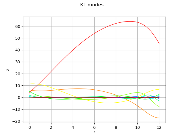
scaledModes = KLResult.getScaledModesAsProcessSample()

[10]:

graph = scaledModes.drawMarginal(0)
graph.setTitle('KL modes')
graph.setXTitle(r'$t$')
graph.setYTitle(r'$z$')
graph

[10]:

../../_images/examples_meta_modeling_viscous_fall_metamodel_19_0.png

We create the postProcessingKL function which takes coefficients of the the K.-L. modes as inputs and returns the trajectories.

[11]:

karhunenLoeveLiftingFunction = ot.KarhunenLoeveLifting(KLResult)

The project method computes the projection of the output sample (i.e. the trajectories) onto the K.-L. modes.

[12]:

outputSampleChaos = KLResult.project(outputSample)

We limit the sampling size of the Kolmogorov selection in order to reduce the computational burden.

[13]:

ot.ResourceMap.SetAsUnsignedInteger("FittingTest-KolmogorovSamplingSize", 1)

We create a polynomial chaos metamodel which takes the input sample and returns the K.-L. modes.

[14]:

algo = ot.FunctionalChaosAlgorithm(inputSample, outputSampleChaos)
algo.run()
chaosMetamodel = algo.getResult().getMetaModel()

The final metamodel is a composition of the KL lifting function and the polynomial chaos metamodel. In order to combine these two functions, we use the PointToFieldConnection class.

[15]:

metaModel = ot.PointToFieldConnection(karhunenLoeveLiftingFunction, chaosMetamodel)

Validate the metamodel¶

Create a validation sample.

[16]:

size = 10
validationInputSample = distribution.getSample(size)
validationOutputSample = alti(validationInputSample)

[17]:

graph = validationOutputSample.drawMarginal(0)
graph.setColors(['red'])
graph2 = metaModel(validationInputSample).drawMarginal(0)
graph2.setColors(['blue'])
graph.add(graph2)
graph.setTitle('Model/metamodel comparison')
graph.setXTitle(r'$t$')
graph.setYTitle(r'$z$')
graph

[17]:

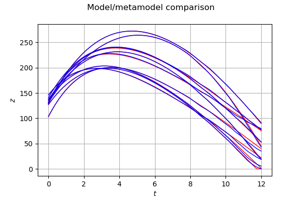
../../_images/examples_meta_modeling_viscous_fall_metamodel_33_0.png

We see that the blue trajectories (i.e. the metamodel) are close to the red trajectories (i.e. the validation sample). This shows that the metamodel is quite accurate. However, we observe that the trajectory singularity that occurs when the object touches the ground (i.e. when $z$ is equal to zero), makes the metamodel less accurate.

OpenTURNS

An Open source initiative for the Treatment of Uncertainties, Risks'N Statistics

Table of Contents

Previous topic

Next topic

This Page