Central tendency analysis on the cantilever beam example
In this example we perform a central tendency analysis of a random variable Y using the various methods available. We consider the cantilever beam example and show how to use the TaylorExpansionMoments and ExpectationSimulationAlgorithm classes.
[1]:
from __future__ import print_function
import openturns as ot
Create the random variable of interest Y=g(X).
[2]:
mean = [50.0, 1.0, 10.0, 5.0]
dim = len(mean)
sigma = ot.Point(dim, 1.0)
R = ot.IdentityMatrix(dim)
distribution = ot.Normal(mean, sigma, R)
X = ot.RandomVector(distribution)
X.setDescription(['E', 'F', 'L', 'I'])
f = ot.SymbolicFunction(['E', 'F', 'L', 'I'], ['F*L^3/(3*E*I)'])
Y = ot.CompositeRandomVector(f, X)
Y.setDescription('Y')
Taylor expansion
Perform Taylor approximation to get the expected value of Y and the importance factors.
[3]:
taylor = ot.TaylorExpansionMoments(Y)
taylor_mean_fo = taylor.getMeanFirstOrder()
taylor_mean_so = taylor.getMeanSecondOrder()
taylor_cov = taylor.getCovariance()
taylor_if = taylor.getImportanceFactors()
print('model evaluation calls number=', f.getGradientCallsNumber())
print('model gradient calls number=', f.getGradientCallsNumber())
print('model hessian calls number=', f.getHessianCallsNumber())
print('taylor mean first order=', taylor_mean_fo)
print('taylor variance=', taylor_cov)
print('taylor importance factors=', taylor_if)
model evaluation calls number= 1
model gradient calls number= 1
model hessian calls number= 1
taylor mean first order= [1.33333]
taylor variance= [[ 2.0096 ]]
taylor importance factors= [E : 0.000353857, F : 0.884642, L : 0.079618, I : 0.0353857]
[4]:
taylor.drawImportanceFactors()
[4]:
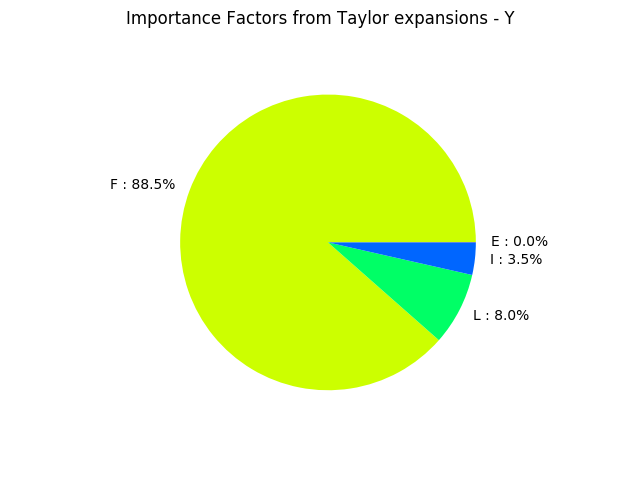
We see that, at first order, the variable  explains 88.5% of the variance of the output
  . On the other hand, the variable
  is not significant in the variance of the output: at first order, the random variable could be replaced by a constant with no change to the output variance.
Monte-Carlo simulation
Perform a Monte Carlo simulation of Y to estimate its mean.
[5]:
algo = ot.ExpectationSimulationAlgorithm(Y)
algo.setMaximumOuterSampling(1000)
algo.setCoefficientOfVariationCriterionType('NONE')
algo.run()
print('model evaluation calls number=', f.getEvaluationCallsNumber())
expectation_result = algo.getResult()
expectation_mean = expectation_result.getExpectationEstimate()
print('monte carlo mean=', expectation_mean, 'var=', expectation_result.getVarianceEstimate())
model evaluation calls number= 1001
monte carlo mean= [1.39543] var= [0.00271142]
Central dispersion analysis based on a sample
Directly compute statistical moments based on a sample of Y. Sometimes the probabilistic model is not available and the study needs to start from the data.
[6]:
Y_s = Y.getSample(1000)
y_mean = Y_s.computeMean()
y_stddev = Y_s.computeStandardDeviationPerComponent()
y_quantile_95p = Y_s.computeQuantilePerComponent(0.95)
print('mean=', y_mean, 'stddev=', y_stddev, 'quantile@95%', y_quantile_95p)
mean= [1.3887] stddev= [1.61762] quantile@95% [4.21421]
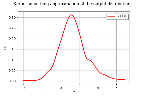
[7]:
graph = ot.KernelSmoothing().build(Y_s).drawPDF()
graph.setTitle("Kernel smoothing approximation of the output distribution")
graph
[7]: