Calibration of the logistic model

We present a calibration study of the logistic growth model defined here.

Analysis of the data

import openturns as ot
import numpy as np
import openturns.viewer as viewer
from matplotlib import pylab as plt
ot.Log.Show(ot.Log.NONE)

We load the logistic model from the usecases module :

from openturns.usecases import logistic_model as logistic_model
lm = logistic_model.LogisticModel()

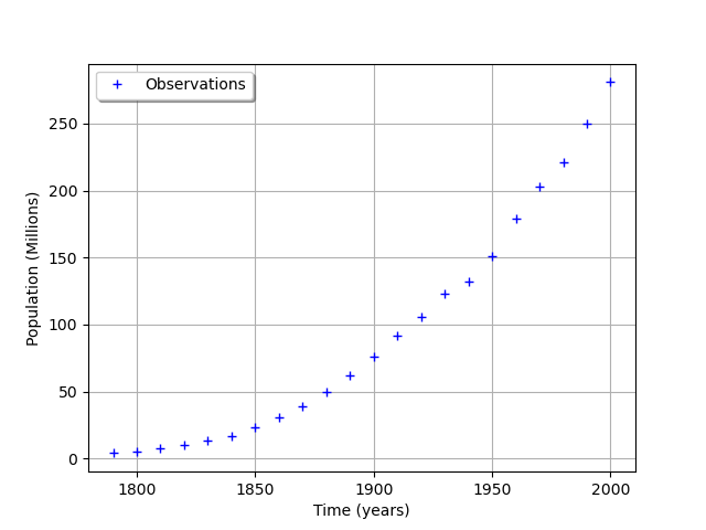
The data is based on 22 dates from 1790 to 2000. The observation points are stored in the data field :

observedSample = lm.data

nbobs = observedSample.getSize()
nbobs

Out:

22

timeObservations = observedSample[:,0]
timeObservations[0:5]

	v0
0	1790
1	1800
2	1810
3	1820
4	1830

populationObservations = observedSample[:,1]
populationObservations[0:5]

	v1
0	3.9
1	5.3
2	7.2
3	9.6
4	13

graph = ot.Graph('', 'Time (years)', 'Population (Millions)', True, 'topleft')
cloud = ot.Cloud(timeObservations, populationObservations)
cloud.setLegend("Observations")
graph.add(cloud)
view = viewer.View(graph)

We consider the times and populations as dimension 22 vectors. The logisticModel function takes a dimension 24 vector as input and returns a dimension 22 vector. The first 22 components of the input vector contains the dates and the remaining 2 components are and .

nbdates = 22
def logisticModel(X):
    t = [X[i] for i in range(nbdates)]
    a = X[22]
    c = X[23]
    t0 = 1790.
    y0 = 3.9e6
    b = np.exp(c)
    y = ot.Point(nbdates)
    for i in range(nbdates):
        y[i] = a*y0/(b*y0+(a-b*y0)*np.exp(-a*(t[i]-t0)))
    z = y/1.e6 # Convert into millions
    return z

logisticModelPy = ot.PythonFunction(24, nbdates, logisticModel)

The reference values of the parameters.

Because is so small with respect to , we use the logarithm.

np.log(1.5587e-10)

Out:

-22.581998789427587

a=0.03134
c=-22.58
thetaPrior = [a,c]

logisticParametric = ot.ParametricFunction(logisticModelPy,[22,23],thetaPrior)

Check that we can evaluate the parametric function.

populationPredicted = logisticParametric(timeObservations.asPoint())
populationPredicted

[3.9,5.29757,7.17769,9.69198,13.0277,17.4068,23.0769,30.2887,39.2561,50.0977,62.7691,77.0063,92.311,108.001,123.322,137.59,150.3,161.184,170.193,177.442,183.144,187.55]#22

graph = ot.Graph('', 'Time (years)', 'Population (Millions)', True, 'topleft')
# Observations
cloud = ot.Cloud(timeObservations, populationObservations)
cloud.setLegend("Observations")
cloud.setColor("blue")
graph.add(cloud)
# Predictions
cloud = ot.Cloud(timeObservations.asPoint(), populationPredicted)
cloud.setLegend("Predictions")
cloud.setColor("green")
graph.add(cloud)
view = viewer.View(graph)

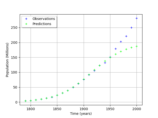
We see that the fit is not good: the observations continue to grow after 1950, while the growth of the prediction seem to fade.

Calibration with linear least squares

timeObservationsVector = ot.Sample([[timeObservations[i,0] for i in range(nbobs)]])
timeObservationsVector[0:10]

	v0	v1	v2	v3	v4	v5	v6	v7	v8	v9	v10	v11	v12	v13	v14	v15	v16	v17	v18	v19	v20	v21
0	1790	1800	1810	1820	1830	1840	1850	1860	1870	1880	1890	1900	1910	1920	1930	1940	1950	1960	1970	1980	1990	2000

populationObservationsVector = ot.Sample([[populationObservations[i, 0] for i in range(nbobs)]])
populationObservationsVector[0:10]

	v0	v1	v2	v3	v4	v5	v6	v7	v8	v9	v10	v11	v12	v13	v14	v15	v16	v17	v18	v19	v20	v21
0	3.9	5.3	7.2	9.6	13	17	23	31	39	50	62	76	92	106	123	132	151	179	203	221	250	281

The reference values of the parameters.

a=0.03134
c=-22.58
thetaPrior = ot.Point([a,c])

logisticParametric = ot.ParametricFunction(logisticModelPy,[22,23],thetaPrior)

Check that we can evaluate the parametric function.

populationPredicted = logisticParametric(timeObservationsVector)
populationPredicted[0:10]

	y0	y1	y2	y3	y4	y5	y6	y7	y8	y9	y10	y11	y12	y13	y14	y15	y16	y17	y18	y19	y20	y21
0	3.9	5.297571	7.177694	9.691977	13.02769	17.40682	23.07691	30.2887	39.25606	50.09767	62.76907	77.0063	92.31103	108.0009	123.3223	137.5899	150.3003	161.1843	170.193	177.4422	183.1443	187.5496

Calibration

algo = ot.LinearLeastSquaresCalibration(logisticParametric, timeObservationsVector, populationObservationsVector, thetaPrior)

algo.run()

calibrationResult = algo.getResult()

thetaMAP = calibrationResult.getParameterMAP()
thetaMAP

[0.0265958,-23.1714]

thetaPosterior = calibrationResult.getParameterPosterior()
thetaPosterior.computeBilateralConfidenceIntervalWithMarginalProbability(0.95)[0]

[0.0246465, 0.028545]
[-23.3182, -23.0247]

transpose samples to interpret several observations instead of several input/outputs as it is a field model

if calibrationResult.getInputObservations().getSize() == 1:
    calibrationResult.setInputObservations([timeObservations[i] for i in range(nbdates)])
    calibrationResult.setOutputObservations([populationObservations[i] for i in range(nbdates)])
    outputAtPrior = [[calibrationResult.getOutputAtPriorMean()[0, i]] for i in range(nbdates)]
    outputAtPosterior = [[calibrationResult.getOutputAtPosteriorMean()[0, i]] for i in range(nbdates)]
    calibrationResult.setOutputAtPriorAndPosteriorMean(outputAtPrior, outputAtPosterior)

graph = calibrationResult.drawObservationsVsInputs()
view = viewer.View(graph)

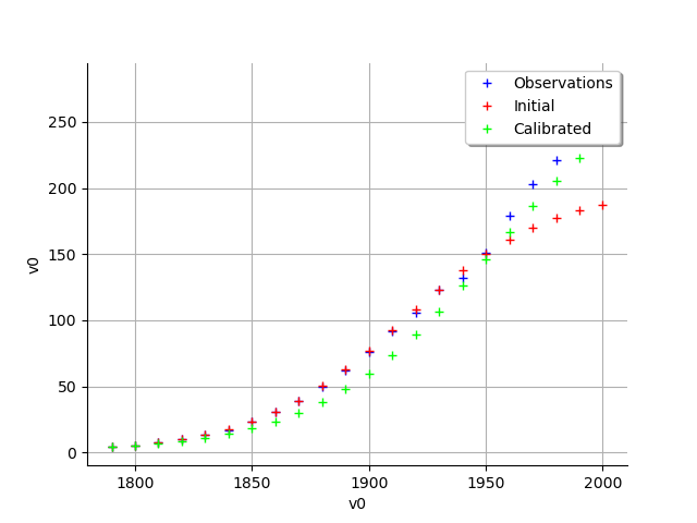
graph = calibrationResult.drawObservationsVsInputs()
view = viewer.View(graph)

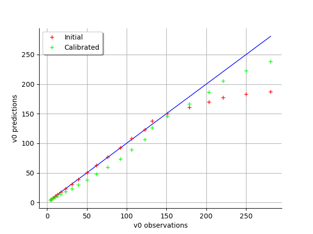
graph = calibrationResult.drawObservationsVsPredictions()
view = viewer.View(graph)

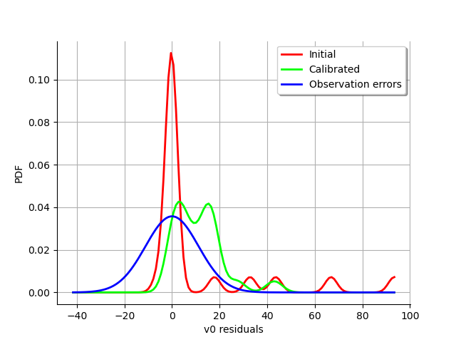
graph = calibrationResult.drawResiduals()
view = viewer.View(graph)

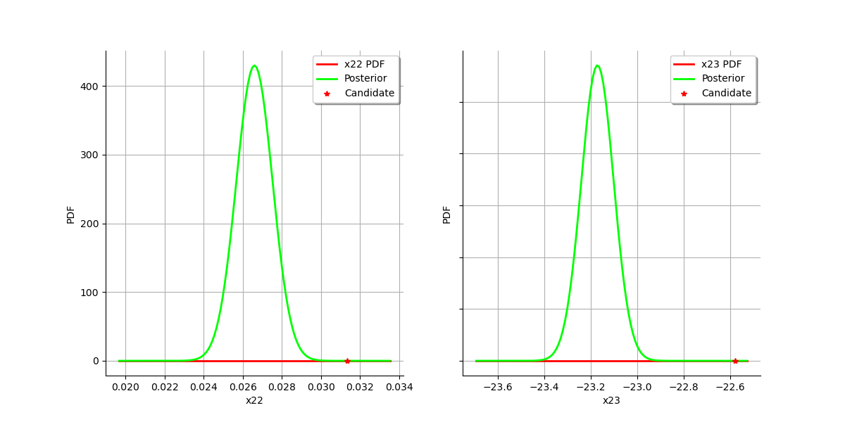
graph = calibrationResult.drawParameterDistributions()
view = viewer.View(graph)

plt.show()