Fit a non parametric distribution

In this example we are going to estimate a non parametric distribution using the kernel smoothing method. After a short introductory example we focus on a few basic features of the API :

• kernel selection

• bandwidth estimation

• an advanced feature such as boundary corrections

from __future__ import print_function
import openturns as ot
import openturns.viewer as viewer
from matplotlib import pylab as plt

ot.Log.Show(ot.Log.NONE)

An introductory example

We create the data from a Gamma distribution :

ot.RandomGenerator.SetSeed(0)
distribution = ot.Gamma(6.0, 1.0)
sample = distribution.getSample(800)

We define the kernel smoother and build the smoothed estimate.

kernel = ot.KernelSmoothing()
estimated = kernel.build(sample)

We can draw the original distribution vs the kernel smoothing.

graph = distribution.drawPDF()
graph.setTitle("Kernel smoothing vs original")
kernel_plot = estimated.drawPDF().getDrawable(0)
kernel_plot.setColor("blue")
graph.add(kernel_plot)
graph.setLegends(["original", "KS"])
graph.setLegendPosition("topright")
view = viewer.View(graph)

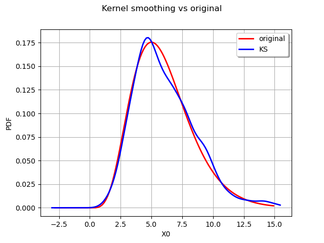
We can obtain the bandwdth parameter :

print(kernel.getBandwidth())

Out:

[0.529581]

We now compute a better bandwitdh with the Silverman rule.

bandwidth = kernel.computeSilvermanBandwidth(sample)
print(bandwidth)

Out:

[0.639633]

The new bandwidth is used to regenerate another fitted distribution :

estimated = kernel.build(sample, bandwidth)

graph = distribution.drawPDF()
graph.setTitle("Kernel smoothing vs original")
kernel_plot = estimated.drawPDF().getDrawable(0)
kernel_plot.setColor("blue")
graph.add(kernel_plot)
graph.setLegends(["original", "KS-Silverman"])
graph.setLegendPosition("topright")
view = viewer.View(graph)

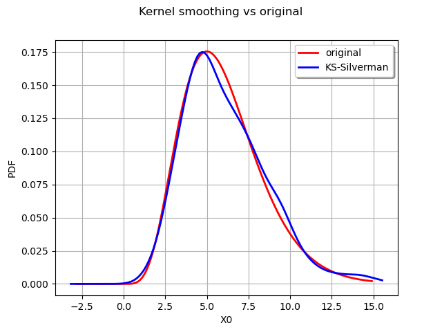
The Silverman rule of thumb to estimate the bandwidth provides a better estimate for the distribution. We can also study the impact of the kernel selection.

Choosing a kernel

We experiment with several kernels to perform the smoothing :

• the standard normal kernel

• the triangular kernel

• the Epanechnikov kernel

• the uniform kernel

We first create the data from a Gamma distribution :

distribution = ot.Gamma(6.0, 1.0)
sample = distribution.getSample(800)

The definition of the Normal kernel :

kernelNormal = ot.KernelSmoothing(ot.Normal())
estimatedNormal = kernelNormal.build(sample)

The definition of the Triangular kernel :

kernelTriangular = ot.KernelSmoothing(ot.Triangular())
estimatedTriangular = kernelTriangular.build(sample)

The definition of the Epanechnikov kernel :

kernelEpanechnikov = ot.KernelSmoothing(ot.Epanechnikov())
estimatedEpanechnikov = kernelEpanechnikov.build(sample)

The definition of the Uniform kernel :

kernelUniform = ot.KernelSmoothing(ot.Uniform())
estimatedUniform = kernelUniform.build(sample)

We finally compare all the distributions :

graph = distribution.drawPDF()
graph.setTitle("Different kernel smoothings vs original distribution")
graph.setGrid(True)

kernel_estimatedNormal_plot = estimatedNormal.drawPDF().getDrawable(0)
kernel_estimatedNormal_plot.setColor("blue")
graph.add(kernel_estimatedNormal_plot)

kernel_estimatedTriangular_plot = estimatedTriangular.drawPDF().getDrawable(0)
kernel_estimatedTriangular_plot.setColor("green")
graph.add(kernel_estimatedTriangular_plot)

kernel_estimatedEpanechnikov_plot = estimatedEpanechnikov.drawPDF().getDrawable(0)
kernel_estimatedEpanechnikov_plot.setColor("orange")
graph.add(kernel_estimatedEpanechnikov_plot)

kernel_estimatedUniform_plot = estimatedUniform.drawPDF().getDrawable(0)
kernel_estimatedUniform_plot.setColor("black")
kernel_estimatedUniform_plot.setLineStyle("dashed")
graph.add(kernel_estimatedUniform_plot)

graph.setLegends(
    ["original", "KS-Normal", "KS-Triangular", "KS-Epanechnikov", "KS-Uniform"]
)

view = viewer.View(graph)

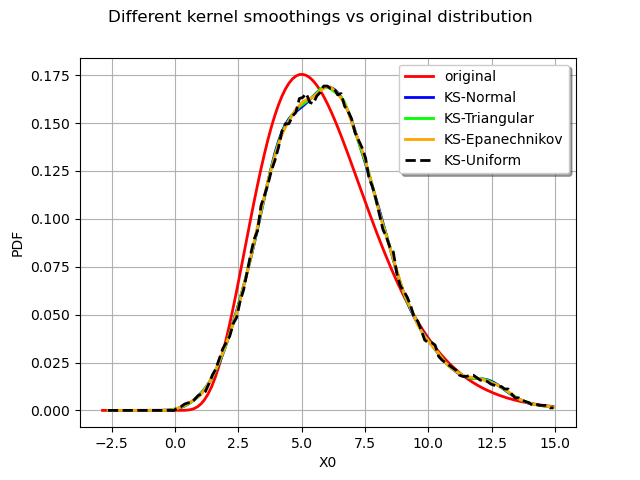
We observe that all the kernels produce very similar results in practice. The Uniform kernel may be seen as the worst of them all while the Epanechnikov one is said to be a good theoritical choice. In practice the standard normal kernel is a fine choice. The most important aspect of kernel smoothing is the choice of the bandwith.

Bandwidth selection

We reproduce a classical example of the literature : the fitting of a bimodal distribution. We will show the result of a kernel smoothing with different bandwidth computation :

• the Silverman rule

• the Plugin bandwidth

• the Mixed bandwidth

We define the bimodal distribution and generate a sample out of it.

X1 = ot.Normal(10.0, 1.0)
X2 = ot.Normal(-10.0, 1.0)
myDist = ot.Mixture([X1, X2])
sample = myDist.getSample(2000)

We now compare the fitted distribution :

graph = myDist.drawPDF()
graph.setTitle("Kernel smoothing vs original")

With the Silverman rule :

kernelSB = ot.KernelSmoothing()
bandwidthSB = kernelSB.computeSilvermanBandwidth(sample)
estimatedSB = kernelSB.build(sample, bandwidthSB)
kernelSB_plot = estimatedSB.drawPDF().getDrawable(0)
graph.add(kernelSB_plot)

With the Plugin bandwidth :

kernelPB = ot.KernelSmoothing()
bandwidthPB = kernelPB.computePluginBandwidth(sample)
estimatedPB = kernelPB.build(sample, bandwidthPB)
kernelPB_plot = estimatedPB.drawPDF().getDrawable(0)
graph.add(kernelPB_plot)

With the Mixed bandwidth :

kernelMB = ot.KernelSmoothing()
bandwidthMB = kernelMB.computeMixedBandwidth(sample)
estimatedMB = kernelMB.build(sample, bandwidthMB)
kernelMB_plot = estimatedMB.drawPDF().getDrawable(0)
kernelMB_plot.setLineStyle("dashed")
graph.add(kernelMB_plot)

graph.setLegends(["original", "KS-Silverman", "KS-Plugin", "KS-Mixed"])
graph.setColors(["red", "blue", "green", "black"])
graph.setLegendPosition("topright")
view = viewer.View(graph)

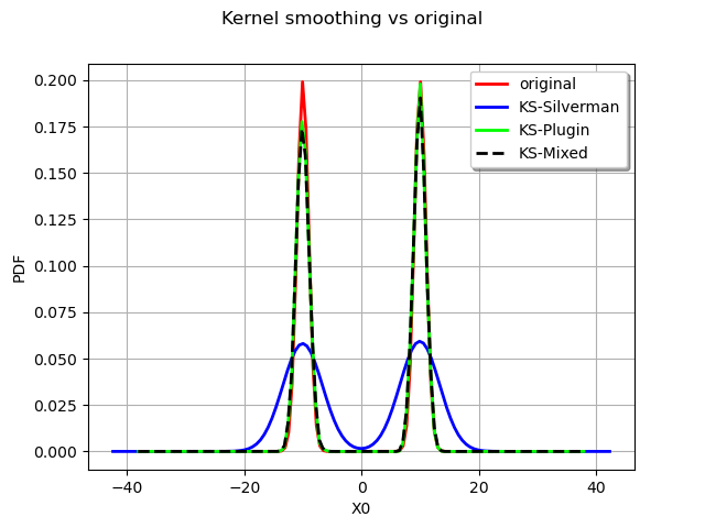
As expected the Silverman seriously overfit the data and the other rules are more to the point.

Boundary corrections

We finish this example on an advanced feature of the kernel smoothing, the boundary corrections.

We consider a Weibull distribution :

myDist = ot.WeibullMin(2.0, 1.5, 1.0)

We generate a sample from the defined distribution :

sample = myDist.getSample(2000)

We draw the exact Weibull distribution :

graph = myDist.drawPDF()

We use two different kernels :

• a standard normal kernel

• the same kernel with a boundary correction

The first kernel without the boundary corrections.

kernel1 = ot.KernelSmoothing()
estimated1 = kernel1.build(sample)

The second kernel with the boundary corrections.

kernel2 = ot.KernelSmoothing()
kernel2.setBoundaryCorrection(True)
estimated2 = kernel2.build(sample)

We compare the estimated PDFs :

graph.setTitle("Kernel smoothing vs original")

kernel1_plot = estimated1.drawPDF().getDrawable(0)
kernel1_plot.setColor("blue")
graph.add(kernel1_plot)

kernel2_plot = estimated2.drawPDF().getDrawable(0)
kernel2_plot.setColor("green")
graph.add(kernel2_plot)


graph.setLegends(["original", "KS", "KS with boundary correction"])
graph.setLegendPosition("topright")
view = viewer.View(graph)

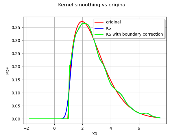
The boundary correction made has a remarkable impact on the quality of the estimate for the small values.

plt.show()