Note
Click here to download the full example code
Estimate a spectral density function
The objective of this example is to estimate the spectral density
function  from data, which can be a sample of time series or one time
series.
from data, which can be a sample of time series or one time
series.
The following example illustrates the case where the available data is a
sample of  realizations of the process, defined on the time grid
![[0, 102.3]](../../_images/math/e97913dfd91a5cd40c71e2c9a98d9e4fea611647.svg) , discretized every
, discretized every  . The spectral model of
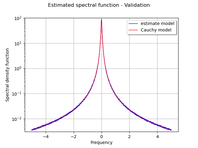
the process is the Cauchy model parameterized by
. The spectral model of
the process is the Cauchy model parameterized by  and
and  .
.
The figure draws the graph of the real spectral model and its estimation from the sample of time series.
from __future__ import print_function
import openturns as ot
import openturns.viewer as viewer
from matplotlib import pylab as plt
ot.Log.Show(ot.Log.NONE)
generate some data
# Create the time grid
# In the context of the spectral estimate or Fourier transform use,
# we use data blocs with size of form 2^p
tMin = 0.
tstep = 0.1
size = 2**12
tgrid = ot.RegularGrid(tMin, tstep, size)

# We fix the parameter of the Cauchy model
amplitude = [5.0]
scale = [3.0]
model = ot.CauchyModel(amplitude, scale)
process = ot.SpectralGaussianProcess(model, tgrid)

# Get a time series or a sample of time series
tseries = process.getRealization()
sample = process.getSample(1000)
Build a spectral model factory
segmentNumber = 10
overlapSize = 0.3
factory = ot.WelchFactory(ot.Hanning(), segmentNumber, overlapSize)
Estimation on a TimeSeries or on a ProcessSample
estimatedModel_TS = factory.build(tseries)
estimatedModel_PS = factory.build(sample)
Change the filtering window
factory.setFilteringWindows(ot.Hamming())
Get the frequencyGrid
frequencyGrid = ot.SpectralGaussianProcess(estimatedModel_PS, tgrid).getFrequencyGrid()
# With the model, we want to compare values
# We compare values computed with theoritical values
plotSample = ot.Sample(frequencyGrid.getN(), 3)

# Loop of comparison ==> data are saved in plotSample
for k in range(frequencyGrid.getN()):
    freq = frequencyGrid.getStart() + k * frequencyGrid.getStep()
    plotSample[k, 0] = freq
    plotSample[k, 1] = abs(estimatedModel_PS(freq)[0, 0])
    plotSample[k, 2] = abs(model(freq)[0, 0])

# Some cosmetics : labels, legend position, ...
graph = ot.Graph("Estimated spectral function - Validation", "Frequency",
              "Spectral density function", True, "topright", 1.0, ot.GraphImplementation.LOGY)

# The first curve is the estimate density as function of frequency
curve1 = ot.Curve(plotSample.getMarginal([0, 1]))
curve1.setColor('blue')
curve1.setLegend('estimate model')

# The second curve is the theoritical density as function of frequency
curve2 = ot.Curve(plotSample.getMarginal([0, 2]))
curve2.setColor('red')
curve2.setLegend('Cauchy model')

graph.add(curve1)
graph.add(curve2)
view = viewer.View(graph)
plt.show()
Total running time of the script: ( 0 minutes 1.367 seconds)