Note
Click here to download the full example code
Estimate Wilks and empirical quantile
In this example we want to evaluate a particular quantile, with the empirical estimator or the Wilks one, from a sample of a random variable.
Let us suppose we want to estimate the quantile  of order
  of the variable
  :
:
 , from the sample
  of size
  , with a confidence level equal to
  .
.
We note  the sample where the values are sorted in ascending order.
The empirical estimator, noted
the sample where the values are sorted in ascending order.
The empirical estimator, noted  , and its confidence interval, is defined by the expressions:
![\left\{
\begin{array}{lcl}
q_{\alpha}^{emp} & = & Y^{(E[n\alpha])} \\
P(q_{\alpha} \in [Y^{(i_n)}, Y^{(j_n)}]) & = & \beta \\
i_n & = & E[n\alpha - a_{\alpha}\sqrt{n\alpha(1-\alpha)}] \\
i_n & = & E[n\alpha + a_{\alpha}\sqrt{n\alpha(1-\alpha)}]
\end{array}
\right\}](../../_images/math/12aa72ea4973557d39876146b62da9c5e666d6b7.svg)
The Wilks estimator, noted  , and its confidence interval, is defined by the expressions:

Once the order  has been chosen, the Wilks number
  is evaluated,
thanks to the static method
is evaluated,
thanks to the static method  of the Wilks object.
In the example, we want to evaluate a quantile  ,
with a confidence level of
,
with a confidence level of  thanks to the
  ).
).
Be careful:  means that the Wilks estimator is the maximum of the sample:
it corresponds to the first maximum of the sample.
means that the Wilks estimator is the maximum of the sample:
it corresponds to the first maximum of the sample.
from __future__ import print_function
import openturns as ot
import math as m
import openturns.viewer as viewer
from matplotlib import pylab as plt
ot.Log.Show(ot.Log.NONE)
model = ot.SymbolicFunction(['x1', 'x2'], ['x1^2+x2'])
R = ot.CorrelationMatrix(2)
R[0,1] = -0.6
inputDist = ot.Normal([0.,0.], R)
inputDist.setDescription(['X1','X2'])
inputVector = ot.RandomVector(inputDist)

# Create the output random vector Y=model(X)
output = ot.CompositeRandomVector(model, inputVector)
Quantile level
alpha = 0.95

# Confidence level of the estimation
beta = 0.90
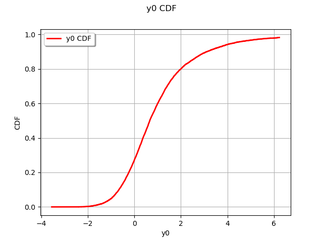
Get a sample of the variable
N = 10**4
sample = output.getSample(N)
graph = ot.UserDefined(sample).drawCDF()
view = viewer.View(graph)
Empirical Quantile Estimator
empiricalQuantile = sample.computeQuantile(alpha)

# Get the indices of the confidence interval bounds
aAlpha = ot.Normal(1).computeQuantile((1.0+beta)/2.0)[0]
min_i = int(N*alpha - aAlpha*m.sqrt(N*alpha*(1.0-alpha)))
max_i = int(N*alpha + aAlpha*m.sqrt(N*alpha*(1.0-alpha)))
#print(min_i, max_i)

# Get the sorted sample
sortedSample = sample.sort()

# Get the Confidence interval of the Empirical Quantile Estimator [infQuantile, supQuantile]
infQuantile = sortedSample[min_i-1]
supQuantile = sortedSample[max_i-1]
print(infQuantile, empiricalQuantile, supQuantile)
Out:
[4.13903] [4.28037] [4.35925]
Wilks number
i = N - (min_i+max_i)//2 # compute wilks with the same sample size
wilksNumber = ot.Wilks.ComputeSampleSize(alpha, beta, i)
print('wilksNumber =', wilksNumber)
Out:
wilksNumber = 10604
Wilks Quantile Estimator
algo = ot.Wilks(output)
wilksQuantile = algo.computeQuantileBound(alpha, beta, i)
print('wilks Quantile 0.95 =', wilksQuantile)
Out:
wilks Quantile 0.95 = [4.37503]
Total running time of the script: ( 0 minutes 0.108 seconds)