The Kolmogorov-Smirnov statistics

In this example, we illustrate how the Kolmogorov-Smirnov statistics is computed.

• We generate a sample from a gaussian distribution.

• We create a Uniform distribution which parameters are estimated from the sample.

• The Kolmogorov-Smirnov statistics is computed and plot on the empirical cumulated distribution function.

import openturns as ot
import openturns.viewer as viewer
from matplotlib import pylab as plt
ot.Log.Show(ot.Log.NONE)

The computeKSStatisticsIndex function computes the Kolmogorov-Smirnov distance between the sample and the distribution. Furthermore, it returns the index which achieves the maximum distance in the sorted sample. The following function is for teaching purposes only: use FittingTest for real applications.

def computeKSStatisticsIndex(sample,distribution):
    sample = ot.Sample(sample.sort())
    n = sample.getSize()
    D = 0.
    index = -1
    D_previous = 0.
    for i in range(n):
        F = distribution.computeCDF(sample[i])
        D = max(F - float(i)/n,float(i+1)/n - F,D)
        if (D > D_previous):
            index = i
            D_previous = D
    return D, index

The drawKSDistance function plots the empirical distribution function of the sample and the Kolmogorov-Smirnov distance at point x.

def drawKSDistance(sample,distribution,x,D,distFactory):
    graph = ot.Graph("KS Distance = %.4f" % (D),"X","CDF",True,"topleft")
    # Vertical line at point x
    ECDF_index = sample.computeEmpiricalCDF([x])
    CDF_index = distribution.computeCDF(x)
    curve = ot.Curve([x,x],[ECDF_index,CDF_index])
    curve.setColor("green")
    curve.setLegend("KS Statistics")
    curve.setLineWidth(4.*curve.getLineWidth())
    graph.add(curve)
    # Empirical CDF
    empiricalCDF = ot.UserDefined(sample).drawCDF()
    empiricalCDF.setColors(["blue"])
    empiricalCDF.setLegends(["Empirical DF"])
    graph.add(empiricalCDF)
    #
    distname = distFactory.getClassName()
    distribution = distFactory.build(sample)
    cdf = distribution.drawCDF()
    cdf.setLegends([distname])
    graph.add(cdf)
    return graph

We generate a sample from a standard gaussian distribution.

N = ot.Normal()
n = 10
sample = N.getSample(n)

Compute the index which achieves the maximum Kolmogorov-Smirnov distance.

We then create a Uniform distribution which parameters are estimated from the sample. This way, the K.S. distance is large enough to being graphically significant.

distFactory = ot.UniformFactory()
distribution = distFactory.build(sample)
distribution

Uniform(a = -1.14233, b = 1.16895)

Compute the index which achieves the maximum Kolmogorov-Smirnov distance.

D, index = computeKSStatisticsIndex(sample,distribution)
print("D=",D,", Index=",index)

Out:

D= 0.23361555328623634 , Index= 2

Get the value which maximizes the distance.

x = sample[index,0]
x

Out:

-0.9772385896485316

graph = drawKSDistance(sample,distribution,x,D,distFactory)
view = viewer.View(graph)
plt.show()

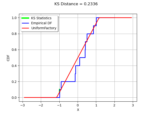
We see that the K.S. statistics is acheived where the distance between the empirical distribution function of the sample and the candidate distribution is largest.