Function manipulation

In this example we are going to exhibit some of the generic function services such as:

• to ask the dimension of its input and output vectors

• to evaluate itself, its gradient and hessian

• to set a finite difference method for the evaluation of the gradient or the hessian

• to evaluate the number of times the function or its gradient or its hessian have been evaluated

• to disable or enable (enabled by default) the history mechanism

• to disable or enable the cache mechanism

• to get all the values evaluated by the function and the associated inputs with the methods

• to clear the history

• to ask the description of its input and output vectors

• to extract output components

• to get a graphical representation

from __future__ import print_function
import openturns as ot
import openturns.viewer as viewer
from matplotlib import pylab as plt
import math as m
ot.Log.Show(ot.Log.NONE)

Create a vectorial function R ^n –> R^p for example R^2 –> R^2

f = ot.SymbolicFunction(['x1', 'x2'], ['1+2*x1+x2', '2+x1+2*x2'])

# Create a scalar function R --> R
func1 = ot.SymbolicFunction(['x'], ['x^2'])

# Create another function R^2 --> R
func2 = ot.SymbolicFunction(['x', 'y'], ['x*y'])

# Create a vectorial function R ^3 --> R^2
func3 = ot.SymbolicFunction(['x1', 'x2', 'x3'], ['1+2*x1+x2+x3^3', '2+sin(x1+2*x2)-sin(x3) * x3^4'])

# Create a second vectorial function R ^n --> R^p
# for example R^2 --> R^2
g = ot.SymbolicFunction(['x1', 'x2'], ['x1+x2', 'x1^2+2*x2^2'])


def python_eval(X):
    a, b = X
    y = a+b
    return [y]
func4 = ot.PythonFunction(2, 1, python_eval)

Ask for the dimension of the input and output vectors

print(f.getInputDimension())
print(f.getOutputDimension())

Out:

2
2

Enable the history mechanism

f = ot.MemoizeFunction(f)

Evaluate the function at a particular point

x = [1.0] * f.getInputDimension()
y = f(x)
print('x=', x, 'y=', y)

Out:

x= [1.0, 1.0] y= [4,5]

Get the history

samplex = f.getInputHistory()
sampley = f.getOutputHistory()
print('evaluation history = ', samplex,  sampley)

Out:

evaluation history =  0 : [ 1 1 ] 0 : [ 4 5 ]

Clear the history mechanism

f.clearHistory()

Disable the history mechanism

f.disableHistory()

Enable the cache mecanism

f4 = ot.MemoizeFunction(func4)
f4.enableCache()
for i in range(10):
    f4(x)

Get the number of times cached values are reused

f4.getCacheHits()

Out:

9

Evaluate the gradient of the function at a particular point

gradientMatrix = f.gradient(x)
gradientMatrix

[[ 2 1 ]
[ 1 2 ]]

Evaluate the hessian of the function at a particular point

hessianMatrix = f.hessian(x)
hessianMatrix

sheet #0
[[ 0 0 ]
[ 0 0 ]]
sheet #1
[[ 0 0 ]
[ 0 0 ]]

Change the gradient method to a non centered finite difference method

step = [1e-7] * f.getInputDimension()
gradient = ot.NonCenteredFiniteDifferenceGradient(step, f.getEvaluation())
f.setGradient(gradient)
gradient

NonCenteredFiniteDifferenceGradient epsilon : [1e-07,1e-07]

Change the hessian method to a centered finite difference method

step = [1e-7] * f.getInputDimension()
hessian = ot.CenteredFiniteDifferenceHessian(step, f.getEvaluation())
f.setHessian(hessian)
hessian

CenteredFiniteDifferenceHessian epsilon : [1e-07,1e-07]

Get the number of times the function has been evaluated

f.getEvaluationCallsNumber()

Out:

1

Get the number of times the gradient has been evaluated

f.getGradientCallsNumber()

Out:

0

Get the number of times the hessian has been evaluated

f.getHessianCallsNumber()

Out:

0

Get the component i

f.getMarginal(1)

[x1,x2]->[2+x1+2*x2]

Compose two functions : h = f o g

ot.ComposedFunction(f, g)

([x1,x2]->[1+2*x1+x2,2+x1+2*x2])o([x1,x2]->[x1+x2,x1^2+2*x2^2])

Get the valid symbolic constants

ot.SymbolicFunction.GetValidConstants()

[e_ -> Euler's constant (2.71828...),pi_ -> Pi constant (3.14159...)]

Graph 1 : z –> f_2(x_0,y_0,z) for z in [-1.5, 1.5] and y_0 = 2. and z_0 = 2.5 Specify the input component that varies Care : numerotation begins at 0

inputMarg = 2
# Give its variation intervall
zMin = -1.5
zMax = 1.5
# Give the coordinates of the fixed input components
centralPt = [1.0, 2.0, 2.5]
# Specify the output marginal function
# Care : numerotation begins at 0
outputMarg = 1
# Specify the point number of the final curve
ptNb = 101
# Draw the curve!
graph = func3.draw(inputMarg, outputMarg, centralPt, zMin, zMax, ptNb)
view = viewer.View(graph)

Graph 2 : (x,z) –> f_1(x,y_0,z) for x in [-1.5, 1.5], z in [-2.5, 2.5] and y_0 = 2.5 Specify the input components that vary

firstInputMarg = 0
secondInputMarg = 2
# Give their variation interval
inputMin2 = [-1.5, -2.5]
inputMax2 = [1.5, 2.5]
# Give the coordinates of the fixed input components
centralPt = [0.0, 2., 2.5]
# Specify the output marginal function
outputMarg = 1
# Specify the point number of the final curve
ptNb = [101, 101]
graph = func3.draw(firstInputMarg, secondInputMarg,
           outputMarg, centralPt, inputMin2, inputMax2, ptNb)
view = viewer.View(graph)

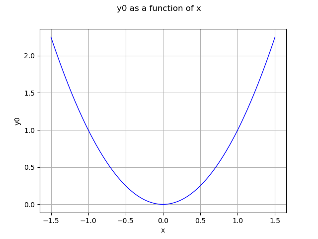
Graph 3 : simplified method for x –> func1(x) for x in [-1.5, 1.5] Give the variation interval

xMin3 = -1.5
xMax3 = 1.5
# Specify the point number of the final curve
ptNb = 101
# Draw the curve!
graph = func1.draw(xMin3, xMax3, ptNb)
view = viewer.View(graph)

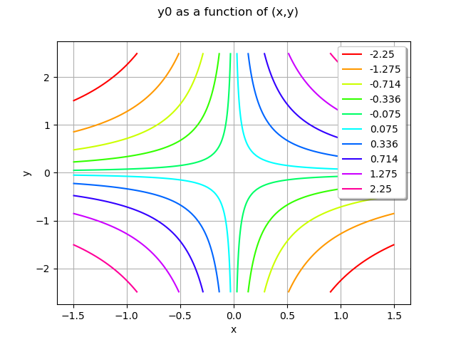
Graph 4 : (x,y) –> func2(x,y) for x in [-1.5, 1.5], y in [-2.5, 2.5] Give their variation interval

inputMin4 = [-1.5, -2.5]
inputMax4 = [1.5, 2.5]
# Give the coordinates of the fixed input components
centralPt = [0.0, 2., 2.5]
# Specify the output marginal function
outputMarg = 1
# Specify the point number of the final curve
ptNb = [101, 101]
graph = func2.draw(inputMin4, inputMax4, ptNb)
view = viewer.View(graph)