Note
Click here to download the full example code
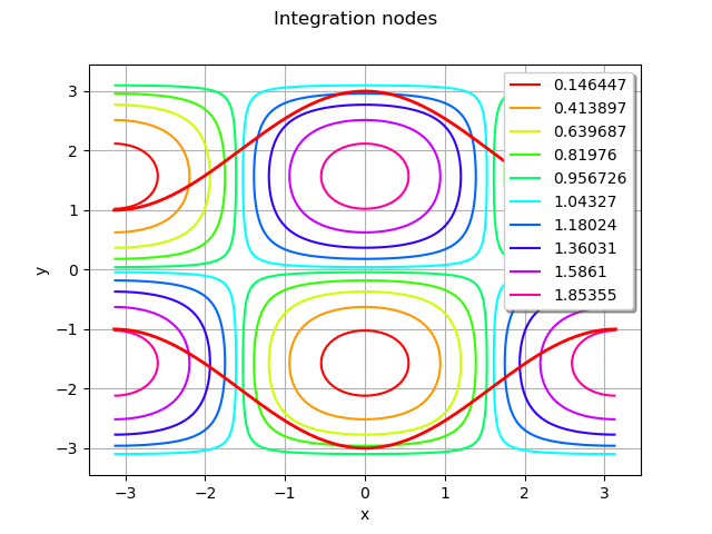
Estimate an integral
In this example we are going to evaluate an integral of the form.

with the iterated quadrature algorithm.
from __future__ import print_function
import openturns as ot
import openturns.viewer as viewer
from matplotlib import pylab as plt
import math as m
ot.Log.Show(ot.Log.NONE)
define the integrand and the bounds
a = -m.pi
b = m.pi
f = ot.SymbolicFunction(['x', 'y'], ['1+cos(x)*sin(y)'])
l = [ot.SymbolicFunction(['x'], [' 2+cos(x)'])]
u = [ot.SymbolicFunction(['x'], ['-2-cos(x)'])]
Draw the graph of the integrand and the bounds
g = ot.Graph('Integration nodes', 'x', 'y', True, 'topright')
g.add(f.draw([a,a],[b,b]))
curve = l[0].draw(a, b).getDrawable(0)
curve.setLineWidth(2)
curve.setColor('red')
g.add(curve)
curve = u[0].draw(a, b).getDrawable(0)
curve.setLineWidth(2)
curve.setColor('red')
g.add(curve)
view = viewer.View(g)
compute the integral value
I2 = ot.IteratedQuadrature().integrate(f, a, b, l, u)
print(I2)
plt.show()
Out:
[-25.1327]
Total running time of the script: ( 0 minutes 0.133 seconds)