Note
Click here to download the full example code
Creation of a regular grid
In this example we will demonstrate how to create a regular grid. Note that a regular grid is a particular mesh of ![\mathcal{D}=[0,T] \in \mathbb{R}](../../_images/math/4b98426bac4949d9956dea99eebd36c085887b27.svg) .
.
Here we will assume it represents the time  as it is often the case, but it can represent any physical quantity.
A regular time grid is a regular discretization of the interval ![[0, T] \in \mathbb{R}](../../_images/math/3eee23f65f3a6c0ef4bf19d4b153bb9345bb58a5.svg) into
into  points, noted
  .
.
The time grid can be defined using  where is the number of points in the time grid.
  the time step between two consecutive instants and
  . Then,
  and
and  .
.
Consider  a multivariate stochastic process of dimension
  , where
  ,
, ![\mathcal{D}=[0,T]](../../_images/math/d4b8ac5329fbacd0712c1e64bca32f52bdc791ef.svg) and
and  is interpreted as a time stamp. Then the mesh associated to the process
  is a (regular) time grid.
from __future__ import print_function
import openturns as ot
import openturns.viewer as viewer
from matplotlib import pylab as plt
import math as m
ot.Log.Show(ot.Log.NONE)
tMin = 0.
tStep = 0.1
n = 10

# Create the grid
time_grid = ot.RegularGrid(tMin, tStep, n)
Get the first and the last instants, the step and the number of points
start = time_grid.getStart()
step = time_grid.getStep()
grid_size = time_grid.getN()
end = time_grid.getEnd()
print('start=', start, 'step=', step, 'grid_size=', grid_size, 'end=', end)
Out:
start= 0.0 step= 0.1 grid_size= 10 end= 1.0
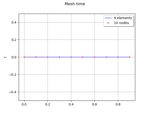
draw the grid
time_grid.setName('time')
graph = time_grid.draw()
view = viewer.View(graph)
plt.show()
Total running time of the script: ( 0 minutes 0.069 seconds)