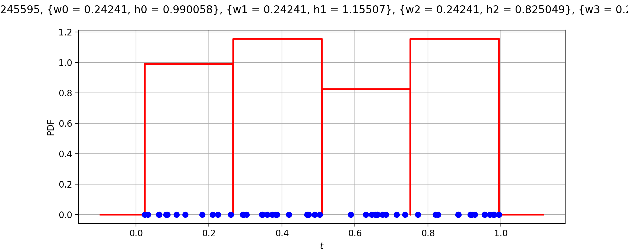
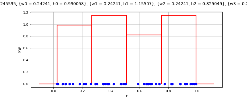
HistogramFactory¶

(Source code, png, hires.png, pdf)

class HistogramFactory(*args)¶

Histogram factory.

Available constructor:: HistogramFactory()

See also

DistributionFactory, Histogram

Notes

The range is $[min(data), max(data)]$ .

See the computeBandwidth method for the bandwidth selection.

Examples

Create an histogram:

>>> import openturns as ot
>>> sample = ot.Normal().getSample(50)
>>> histogram = ot.HistogramFactory().build(sample)

Create an histogram from a number of bins:

>>> import openturns as ot
>>> sample = ot.Normal().getSample(50)
>>> binNumber = 10
>>> histogram = ot.HistogramFactory().build(sample, binNumber)

Create an histogram from a bandwidth:

>>> import openturns as ot
>>> sample = ot.Normal().getSample(50)
>>> bandwidth = 0.5
>>> histogram = ot.HistogramFactory().build(sample, bandwidth)

Create an histogram from a first value and widths:

>>> import openturns as ot
>>> ot.RandomGenerator.SetSeed(0)
>>> sample = ot.Normal().getSample(50)
>>> first = -4
>>> width = ot.Point(7, 1.)
>>> histogram = ot.HistogramFactory().build(sample, first, width)

Compute bandwidth with default robust estimator:

>>> import openturns as ot
>>> ot.RandomGenerator.SetSeed(0)
>>> sample = ot.Normal().getSample(50)
>>> factory = ot.HistogramFactory()
>>> factory.computeBandwidth(sample)
0.8207...

Compute bandwidth with optimal estimator:

>>> import openturns as ot
>>> ot.RandomGenerator.SetSeed(0)
>>> sample = ot.Normal().getSample(50)
>>> factory = ot.HistogramFactory()
>>> factory.computeBandwidth(sample, False)
0.9175...

Methods

`build`(*args)	Build the distribution.
`buildAsHistogram`(*args)	Estimate the distribution as native distribution.
`buildEstimator`(*args)	Build the distribution and the parameter distribution.
`computeBandwidth`(sample[, useQuantile])	Compute the bandwidth.
`getBootstrapSize`()	Accessor to the bootstrap size.
`getClassName`()	Accessor to the object’s name.
`getId`()	Accessor to the object’s id.
`getName`()	Accessor to the object’s name.
`getShadowedId`()	Accessor to the object’s shadowed id.
`getVisibility`()	Accessor to the object’s visibility state.
`hasName`()	Test if the object is named.
`hasVisibleName`()	Test if the object has a distinguishable name.
`setBootstrapSize`(bootstrapSize)	Accessor to the bootstrap size.
`setName`(name)	Accessor to the object’s name.
`setShadowedId`(id)	Accessor to the object’s shadowed id.
`setVisibility`(visible)	Accessor to the object’s visibility state.

__init__(*args)¶: Initialize self. See help(type(self)) for accurate signature.

build(*args)¶

Build the distribution.

Available usages:

build(sample)

build(param)

Parameters

sample2-d sequence of float: Sample from which the distribution parameters are estimated.
paramCollection of PointWithDescription: A vector of parameters of the distribution.

Returns

distDistribution: The built distribution.

buildAsHistogram(*args)¶

Estimate the distribution as native distribution.

If the sample is constant, the range of the histogram would be zero. In this case, the range is set to be a factor of the Distribution-DefaultCDFEpsilon key of the ResourceMap.

Available usages:

build(sample)

build(sample, binNumber)

build(sample, bandwidth)

build(sample, first, width)

Parameters

sampleSample: Data
binNumberint: The number of classes.
bandwidthfloat: The width of each class.
firstfloat: The lower bound of the first class.
width1-d sequence of float: The widths of the classes.

Returns

distributionHistogram: The estimated distribution

buildEstimator(*args)¶

Build the distribution and the parameter distribution.

Parameters

sample2-d sequence of float: Sample from which the distribution parameters are estimated.
parametersDistributionParameters: Optional, the parametrization.

Returns

resDistDistributionFactoryResult: The results.

Notes

According to the way the native parameters of the distribution are estimated, the parameters distribution differs:

Moments method: the asymptotic parameters distribution is normal and estimated by Bootstrap on the initial data;

Maximum likelihood method with a regular model: the asymptotic parameters distribution is normal and its covariance matrix is the inverse Fisher information matrix;

Other methods: the asymptotic parameters distribution is estimated by Bootstrap on the initial data and kernel fitting (see KernelSmoothing).

If another set of parameters is specified, the native parameters distribution is first estimated and the new distribution is determined from it:

if the native parameters distribution is normal and the transformation regular at the estimated parameters values: the asymptotic parameters distribution is normal and its covariance matrix determined from the inverse Fisher information matrix of the native parameters and the transformation;

in the other cases, the asymptotic parameters distribution is estimated by Bootstrap on the initial data and kernel fitting.

computeBandwidth(sample, useQuantile=True)¶

Compute the bandwidth.

The bandwidth of the histogram is based on the asymptotic mean integrated squared error (AMISE).

When useQuantile is True (the default), the bandwidth is based on the quantiles of the sample. For any $\alpha\in(0,1]$ , let $q_n(\alpha)$ be the empirical quantile at level $\alpha$ of the sample. Let $Q_1$ and $Q_3$ be the first and last quartiles of the sample:

$\begin{aligned} Q_3 = q_n(0.75), \qquad Q_1 = q_n(0.25), \end{aligned}$

and let $IQR$ be the inter-quartiles range:

$\begin{aligned} IQR = Q_3 - Q_1. \end{aligned}$

In this case, the bandwidth is the robust estimator of the AMISE-optimal bandwith, known as Freedman and Diaconis rule [freedman1981]:

$\begin{aligned} h = \frac{IQR}{2\Phi^{-1}(0.75)} \left(\frac{24 \sqrt{\pi}}{n}\right)^{\frac{1}{3}} \end{aligned}$

where $\Phi^{-1}$ is the quantile function of the gaussian standard distribution. The expression $\frac{IQR}{2\Phi^{-1}(0.75)}$ is the normalized inter-quartile range and is equal to the standard deviation of the gaussian distribution. The normalized inter-quartile range is a robust estimator of the scale of the distribution (see [wand1994], page 60).

When useQuantile is False, the bandwidth is the AMISE-optimal one, known as Scott’s rule:

$\begin{aligned} h = \sigma_n \left(\frac{24 \sqrt{\pi}}{n}\right)^{\frac{1}{3}} \end{aligned}$

where $\sigma_n^2$ is the unbiaised variance of the data. This estimator is optimal for the gaussian distribution (see [scott1992]). In this case, the AMISE is $O(n^{-2/3})$ .

If the bandwidth is computed as zero (for example, if the sample is constant), then the Distribution-DefaultQuantileEpsilon key of the ResourceMap is used instead.

Parameters

sampleSample: Data

Returns

bandwidthfloat: The estimated bandwidth
useQuantilebool, optional (default=`True`): If True, then use the robust bandwidth estimator based on Freedman and Diaconis rule. Otherwise, use the optimal bandwidth estimator based on Scott’s rule.

getBootstrapSize()¶

Accessor to the bootstrap size.

Returns

sizeinteger: Size of the bootstrap.

getClassName()¶

Accessor to the object’s name.

Returns

class_namestr: The object class name (object.__class__.__name__).

getId()¶

Accessor to the object’s id.

Returns

idint: Internal unique identifier.

getName()¶

Accessor to the object’s name.

Returns

namestr: The name of the object.

getShadowedId()¶

Accessor to the object’s shadowed id.

Returns

idint: Internal unique identifier.

getVisibility()¶

Accessor to the object’s visibility state.

Returns

visiblebool: Visibility flag.

hasName()¶

Test if the object is named.

Returns

hasNamebool: True if the name is not empty.

hasVisibleName()¶

Test if the object has a distinguishable name.

Returns

hasVisibleNamebool: True if the name is not empty and not the default one.

setBootstrapSize(bootstrapSize)¶

Accessor to the bootstrap size.

Parameters

sizeinteger: Size of the bootstrap.

setName(name)¶

Accessor to the object’s name.

Parameters

namestr: The name of the object.

setShadowedId(id)¶

Accessor to the object’s shadowed id.

Parameters

idint: Internal unique identifier.

setVisibility(visible)¶

Accessor to the object’s visibility state.

Parameters

visiblebool: Visibility flag.

OpenTURNS

An Open source initiative for the Treatment of Uncertainties, Risks'N Statistics

Previous topic

Next topic

This Page

HistogramFactory¶