Note
Click here to download the full example code
Estimate correlation coefficients
In this example we are going to estimate the correlation between an output sample Y and the corresponding inputs using various estimators:
Pearson coefficients
Spearman coefficients
PCC: Partial Correlation Coefficients
PRCC: Partial Rank Correlation Coefficient
SRC: Standard Regression Coefficients
SRRC: Standard Rank Regression Coefficient
from __future__ import print_function
import openturns as ot
import openturns.viewer as viewer
from matplotlib import pylab as plt
ot.Log.Show(ot.Log.NONE)
To illustrate the usage of the method mentionned above, we define a set of X/Y data using the Ishigami model. This classical model is defined in a data class :
from openturns.usecases import ishigami_function as ishigami_function
im = ishigami_function.IshigamiModel()
Create X/Y data We get the input variables description :
input_names = im.distributionX.getDescription()

size = 100
inputDesign = ot.SobolIndicesExperiment(im.distributionX, size, True).generate()
outputDesign = im.model(inputDesign)
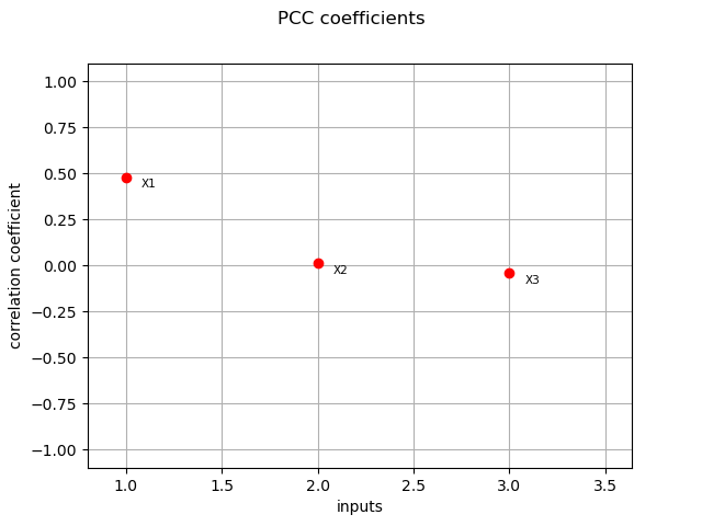
PCC coefficients
We compute here PCC coefficients using the CorrelationAnalysis
pcc_indices = ot.CorrelationAnalysis.PCC(inputDesign, outputDesign)
print(pcc_indices)
Out:
[0.48083,0.0118573,-0.0399335]
graph = ot.SobolIndicesAlgorithm.DrawCorrelationCoefficients(pcc_indices, input_names, "PCC coefficients")
view = viewer.View(graph)
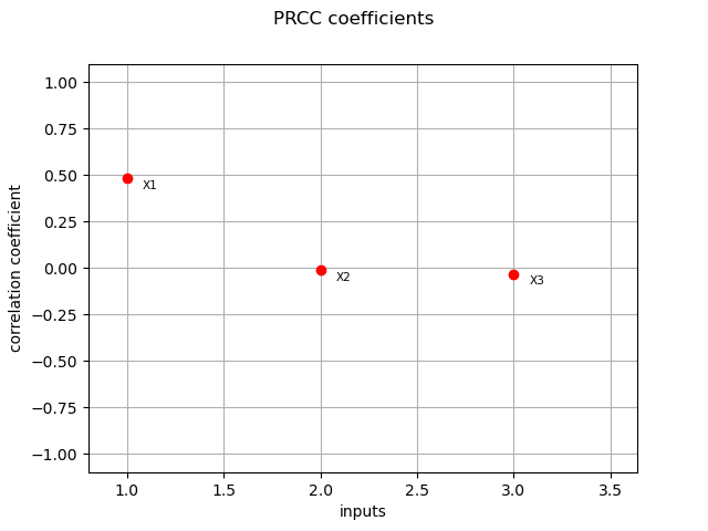
PRCC coefficients
We compute here PRCC coefficients using the CorrelationAnalysis
prcc_indices = ot.CorrelationAnalysis.PRCC(inputDesign, outputDesign)
print(prcc_indices)
Out:
[0.48438,-0.00850357,-0.0310585]
graph = ot.SobolIndicesAlgorithm.DrawCorrelationCoefficients(prcc_indices, input_names, "PRCC coefficients")
view = viewer.View(graph)
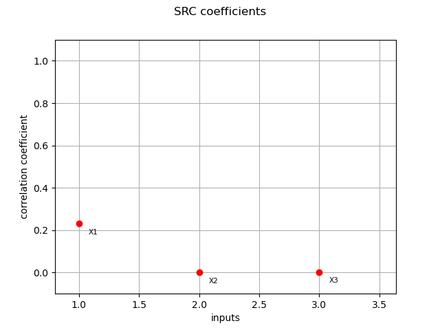
SRC coefficients
We compute here SRC coefficients using the CorrelationAnalysis
src_indices = ot.CorrelationAnalysis.SRC(inputDesign, outputDesign)
print(src_indices)
Out:
[0.231036,0.000107773,0.00122827]
graph = ot.SobolIndicesAlgorithm.DrawCorrelationCoefficients(src_indices, input_names, 'SRC coefficients')
view = viewer.View(graph)
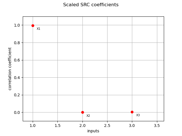
Case where coefficients sum to 1 :
scale_src_indices = ot.CorrelationAnalysis.SRC(inputDesign, outputDesign, True)
print(scale_src_indices)
Out:
[0.99425,0.000463796,0.00528582]
And its associated graph:
graph = ot.SobolIndicesAlgorithm.DrawCorrelationCoefficients(scale_src_indices, input_names, 'Scaled SRC coefficients')
view = viewer.View(graph)
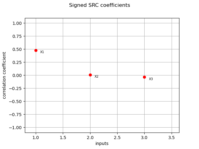
Finally, using signed src: we get the trend importance :
signed_src_indices = ot.CorrelationAnalysis.SignedSRC(inputDesign, outputDesign)
print(signed_src_indices)
Out:
[0.480662,0.0103814,-0.0350468]
and its graph :
graph = ot.SobolIndicesAlgorithm.DrawCorrelationCoefficients(signed_src_indices, input_names, 'Signed SRC coefficients')
view = viewer.View(graph)
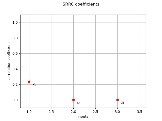
SRRC coefficients
We compute here SRRC coefficients using the CorrelationAnalysis
srrc_indices = ot.CorrelationAnalysis.SRRC(inputDesign, outputDesign)
print(srrc_indices)
Out:
[0.234826,5.52475e-05,0.00074076]
graph = ot.SobolIndicesAlgorithm.DrawCorrelationCoefficients(srrc_indices, input_names, 'SRRC coefficients')
view = viewer.View(graph)
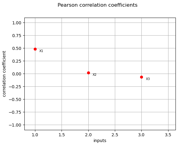
Pearson coefficients
We compute here the Pearson  coefficients using the CorrelationAnalysis
pearson_correlation = ot.CorrelationAnalysis.PearsonCorrelation(inputDesign, outputDesign)
print(pearson_correlation)
Out:
[0.482871,0.0178456,-0.0638373]
graph = ot.SobolIndicesAlgorithm.DrawCorrelationCoefficients(pearson_correlation,
                                                     input_names,
                                                     "Pearson correlation coefficients")
view = viewer.View(graph)
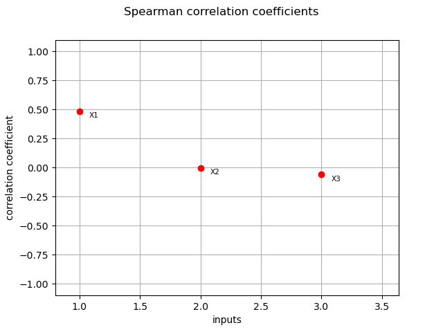
Spearman coefficients
We compute here the Pearson  coefficients using the CorrelationAnalysis
spearman_correlation = ot.CorrelationAnalysis.SpearmanCorrelation(inputDesign, outputDesign)
print(spearman_correlation)
Out:
[0.486298,-0.00194796,-0.0585667]
graph = ot.SobolIndicesAlgorithm.DrawCorrelationCoefficients(spearman_correlation,
                                                     input_names,
                                                     "Spearman correlation coefficients")
view = viewer.View(graph)
plt.show()
Total running time of the script: ( 0 minutes 0.813 seconds)