Select fitted distributions

In this example help to make a choice between several distributions fitted to a sample.

Several methods can be used:

• the ranking by the Kolmogorov p-values (for continuous distributions),

• the ranking by the ChiSquared p-values (for discrete distributions),

• the ranking by BIC values.

from __future__ import print_function
import openturns as ot
import openturns.viewer as viewer
from matplotlib import pylab as plt
ot.Log.Show(ot.Log.NONE)

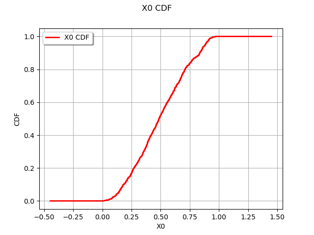
Create a sample from a continuous distribution

distribution = ot.Beta(2.0, 2.0, 0.0, 1.)
sample = distribution.getSample(1000)
graph = ot.UserDefined(sample).drawCDF()
view = viewer.View(graph)

1. Specify the model only

Create the list of distribution estimators

factories = [ot.BetaFactory(), ot.TriangularFactory()]

Rank the continuous models by the Lilliefors p-values:

estimated_distribution, test_result = ot.FittingTest.BestModelLilliefors(sample, factories)
test_result

class=TestResult name=Unnamed type=Lilliefors Beta binaryQualityMeasure=false p-value threshold=0.5 p-value=0.006 statistic=0.0327766 description=[Beta(alpha = 1.72649, beta = 1.66568, a = 0.00526109, b = 0.970313) vs sample Beta]

Rank the continuous models wrt the BIC criteria (no test result):

ot.FittingTest.BestModelBIC(sample, factories)

Out:

[class=Beta name=Beta dimension=1 alpha=1.72649 beta=1.66568 a=0.00526109 b=0.970313, -0.19254944819710879]

Rank the continuous models wrt the AIC criteria (no test result)

ot.FittingTest.BestModelAIC(sample, factories)

Out:

[class=Beta name=Beta dimension=1 alpha=1.72649 beta=1.66568 a=0.00526109 b=0.970313, -0.21218046931303733]

Rank the continuous models wrt the AICc criteria (no test result):

ot.FittingTest.BestModelAICC(sample, factories)

Out:

[class=Beta name=Beta dimension=1 alpha=1.72649 beta=1.66568 a=0.00526109 b=0.970313, -0.2121402683080122]

2. Specify the model and its parameters

Create a collection of the distributions to be tested

distributions = [ot.Beta(2.0, 2.0, 0.0, 1.0), ot.Triangular(0.0, 0.5, 1.0)]

Rank the continuous models by the Kolmogorov p-values:

estimated_distribution, test_result = ot.FittingTest.BestModelKolmogorov(sample, distributions)
test_result

class=TestResult name=Unnamed type=Kolmogorov Beta binaryQualityMeasure=true p-value threshold=0.05 p-value=0.127302 statistic=0.0369407 description=[Beta(alpha = 2, beta = 2, a = 0, b = 1) vs sample Beta]

Rank the continuous models wrt the BIC criteria:

ot.FittingTest.BestModelBIC(sample, distributions)

Out:

[class=Beta name=Beta dimension=1 alpha=2 beta=2 a=0 b=1, -0.21804827501286062]

Rank the continuous models wrt the AIC criteria:

ot.FittingTest.BestModelAIC(sample, distributions)

Out:

[class=Beta name=Beta dimension=1 alpha=2 beta=2 a=0 b=1, -0.21804827501286062]

Rank the continuous models wrt the AICc criteria:

ot.FittingTest.BestModelAICC(sample, distributions)

Out:

[class=Beta name=Beta dimension=1 alpha=2 beta=2 a=0 b=1, -0.21804827501286062]

Discrete distributions

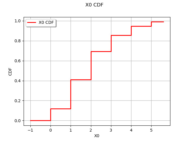
Create a sample from a discrete distribution

distribution = ot.Poisson(2.0)
sample = distribution.getSample(1000)
graph = ot.UserDefined(sample).drawCDF()
view = viewer.View(graph)

Create the list of distribution estimators

distributions = [ot.Poisson(2.0), ot.Geometric(0.1)]

Rank the discrete models wrt the ChiSquared p-values:

estimated_distribution, test_result = ot.FittingTest.BestModelChiSquared(sample, distributions)
test_result

class=TestResult name=Unnamed type=ChiSquared Poisson binaryQualityMeasure=true p-value threshold=0.05 p-value=0.184085 statistic=8.81784 description=[Poisson(lambda = 2) vs sample Poisson]

Rank the discrete models wrt the BIC criteria:

ot.FittingTest.BestModelBIC(sample, distributions)
plt.show()