Note
Click here to download the full example code
Truncate a distribution
In this example we are going to define truncated distributions.
It is possible to truncate a distribution in its lower area, or its upper area or in both lower and upper areas.
In 1-d, assuming a and b bounds, its probability density function is defined as:
Is is also possible to truncate a multivariate distribution.
from __future__ import print_function
import openturns as ot
import openturns.viewer as viewer
from matplotlib import pylab as plt
ot.Log.Show(ot.Log.NONE)

# the original distribution
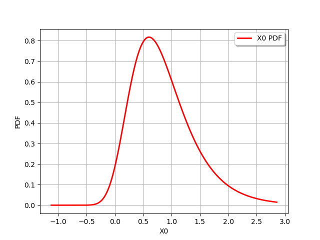
distribution = ot.Gumbel(0.45, 0.6)
graph = distribution.drawPDF()
view = viewer.View(graph)

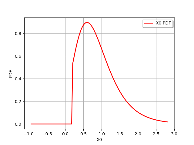
truncate on the left
truncated = ot.TruncatedDistribution(distribution, 0.2, ot.TruncatedDistribution.LOWER)
graph = truncated.drawPDF()
view = viewer.View(graph)

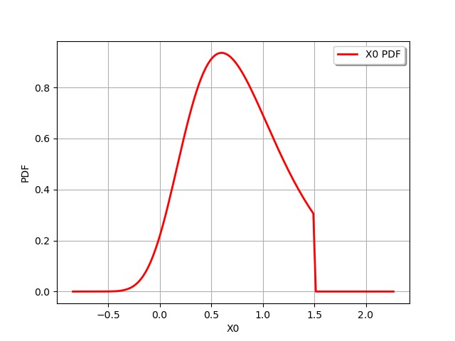
truncate on the right
truncated = ot.TruncatedDistribution(distribution, 1.5, ot.TruncatedDistribution.UPPER)
graph = truncated.drawPDF()
view = viewer.View(graph)

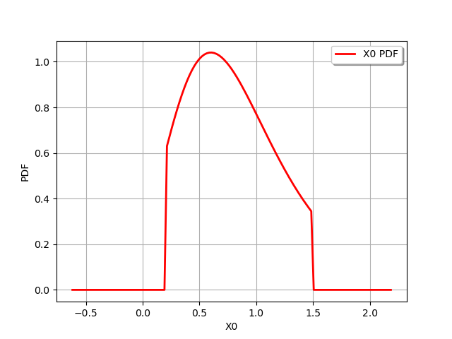
truncated on both bounds
truncated = ot.TruncatedDistribution(distribution, 0.2, 1.5)
graph = truncated.drawPDF()
view = viewer.View(graph)

Define a multivariate distribution
dimension = 2
size = 70
sample = ot.Normal(dimension).getSample(size)
ks = ot.KernelSmoothing().build(sample)
Truncate it between (-2;2)^n
bounds = ot.Interval([-2.0] * dimension, [2.0] * dimension)
truncatedKS = ot.Distribution(ot.TruncatedDistribution(ks, bounds))
Draw its PDF
graph = truncatedKS.drawPDF([-2.5] * dimension, [2.5] * dimension, [256] * dimension)
graph.add(ot.Cloud(truncatedKS.getSample(200)))
graph.setColors(["blue", "red"])
view = viewer.View(graph)
plt.show()
![[X0,X1] iso-PDF](../../_images/sphx_glr_plot_truncated_distribution_005.png)
Out:
/home/devel/project/build/python/src/site-packages/openturns/viewer.py:437: UserWarning: No contour levels were found within the data range.
  contourset = self._ax[0].contour(X, Y, Z, **contour_kw)
Total running time of the script: ( 0 minutes 0.608 seconds)
 OpenTURNS