Note
Click here to download the full example code
Create a mesh
from __future__ import print_function
import openturns as ot
import openturns.viewer as viewer
from matplotlib import pylab as plt
import math as m
ot.Log.Show(ot.Log.NONE)
Creation of a regular grid
In this first part we demonstrate how to create a regular grid. Note that a regular grid is a particular mesh of ![\mathcal{D}=[0,T] \in \mathbb{R}](../../_images/math/4b98426bac4949d9956dea99eebd36c085887b27.svg) .
.
Here we assume it represents the time  as it is often the case, but it can represent any physical quantity.
A regular time grid is a regular discretization of the interval ![[0, T] \in \mathbb{R}](../../_images/math/3eee23f65f3a6c0ef4bf19d4b153bb9345bb58a5.svg) into
into  points, noted
  .
.
The time grid can be defined using  where is the number of points in the time grid.
  the time step between two consecutive instants and
  . Then,
  and
and  .
.
Consider  a multivariate stochastic process of dimension
  , where
  ,
, ![\mathcal{D}=[0,T]](../../_images/math/d4b8ac5329fbacd0712c1e64bca32f52bdc791ef.svg) and
and  is interpreted as a time stamp. Then the mesh associated to the process
  is a (regular) time grid.
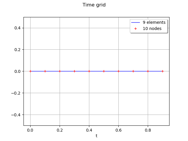
We define a time grid from a starting time tMin, a time step tStep and a number of time steps n.
tMin = 0.
tStep = 0.1
n = 10
time_grid = ot.RegularGrid(tMin, tStep, n)
We get the first and the last instants, the step and the number of points :
start = time_grid.getStart()
step = time_grid.getStep()
grid_size = time_grid.getN()
end = time_grid.getEnd()
print('start=', start, 'step=', step, 'grid_size=', grid_size, 'end=', end)
Out:
start= 0.0 step= 0.1 grid_size= 10 end= 1.0
We draw the grid.
time_grid.setName('time')
graph = time_grid.draw()
graph.setTitle("Time grid")
graph.setXTitle("t")
graph.setYTitle("")
view = viewer.View(graph)
Creation of a mesh
In this paragraph we create a mesh  associated to a domain
  .
.
A mesh is defined from vertices in  and a topology that connects the vertices: the simplices. The simplex
 ![Indices([i_1,\dots, i_{n+1}])](../../_images/math/66e1ad6a8e4df0afde92b24065dcc9036406654e.svg) relies the vertices of index
relies the vertices of index  in
in  . In dimension 1, a simplex is an interval
 ![Indices([i_1,i_2])](../../_images/math/5acc32c3570bde126f2f82611f0e2a72916d65aa.svg) ; in dimension 2, it is a triangle
; in dimension 2, it is a triangle ![Indices([i_1,i_2, i_3])](../../_images/math/0438950cfb533784096e37cead13f0cbe0423c29.svg) .
.
The library enables to easily create a mesh which is a box of dimension  or
or  regularly meshed in all its directions, thanks to the object IntervalMesher.
Consider a multivariate stochastic process of dimension , where . The mesh is a discretization of the domain  .
.
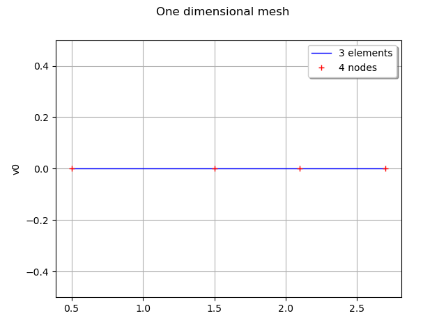
A one dimensional mesh is created and represented by :
vertices = [[0.5], [1.5], [2.1], [2.7]]
simplicies = [[0, 1], [1, 2], [2, 3]]
mesh1D = ot.Mesh(vertices, simplicies)
graph1 = mesh1D.draw()
graph1.setTitle('One dimensional mesh')
view = viewer.View(graph1)
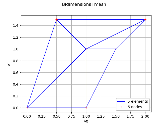
We define a bidimensional mesh :
vertices = [[0.0, 0.0], [1.0, 0.0], [1.0, 1.0], [1.5, 1.0], [2.0, 1.5], [0.5, 1.5]]
simplicies = [[0, 1, 2], [1, 2, 3], [2, 3, 4], [2, 4, 5], [0, 2, 5]]
mesh2D = ot.Mesh(vertices, simplicies)
graph2 = mesh2D.draw()
graph2.setTitle('Bidimensional mesh')
graph2.setLegendPosition('bottomright')
view = viewer.View(graph2)
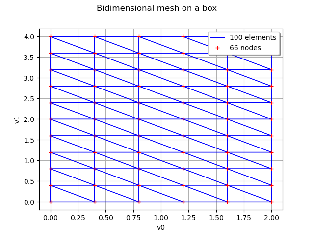
We can also define a mesh which is a regularly meshed box in dimension 1 or 2. We define the number of intervals in each direction of the box :
myIndices = [5, 10]
myMesher = ot.IntervalMesher(myIndices)
We then create the mesh of the box ![[0, 2] \times [0, 4]](../../_images/math/6b060d54ce2a81934d0d5635863b4fbab503b4de.svg) :
:
lowerBound=[0., 0.]
upperBound=[2., 4.]
myInterval = ot.Interval(lowerBound, upperBound)
myMeshBox = myMesher.build(myInterval)
mygraph3 = myMeshBox.draw()
mygraph3.setTitle('Bidimensional mesh on a box')
view = viewer.View(mygraph3)
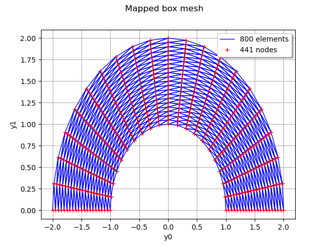
It is possible to perform a transformation on a regularly meshed box.
myIndices = [20, 20]
mesher = ot.IntervalMesher(myIndices)
# r in [1., 2.] and theta in (0., pi]
lowerBound2 = [1.0, 0.0]
upperBound2 = [2.0, m.pi]
myInterval = ot.Interval(lowerBound2, upperBound2)
meshBox2 = mesher.build(myInterval)
We define the mapping function and draw the transformation :
f = ot.SymbolicFunction(['r', 'theta'], ['r*cos(theta)', 'r*sin(theta)'])
oldVertices = meshBox2.getVertices()
newVertices = f(oldVertices)
meshBox2.setVertices(newVertices)
graphMappedBox = meshBox2.draw()
graphMappedBox.setTitle('Mapped box mesh')
view = viewer.View(graphMappedBox)
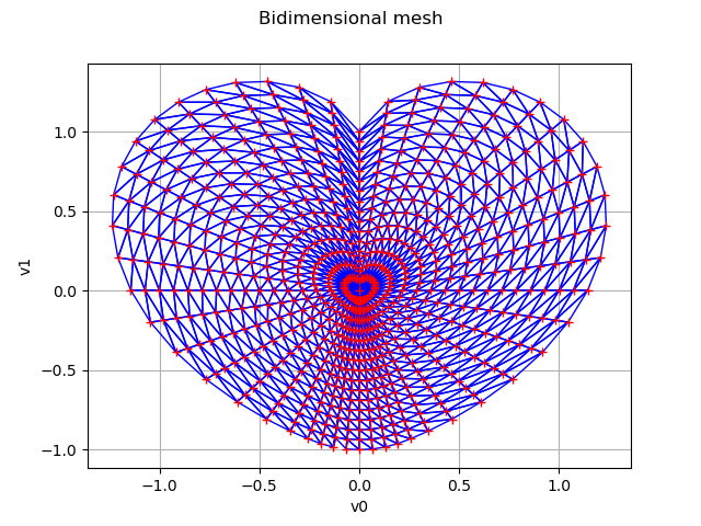
Finally we create a mesh of a heart in dimension 2.
def meshHeart(ntheta, nr):
    # First, build the nodes
    nodes = ot.Sample(0, 2)
    nodes.add([0.0, 0.0])
    for j in range(ntheta):
        theta = (m.pi * j) / ntheta
        if (abs(theta - 0.5 * m.pi) < 1e-10):
            rho = 2.0
        elif (abs(theta) < 1e-10) or (abs(theta-m.pi) < 1e-10):
            rho = 0.0
        else:
            absTanTheta = abs(m.tan(theta))
            rho = absTanTheta**(1.0 / absTanTheta) + m.sin(theta)
        cosTheta = m.cos(theta)
        sinTheta = m.sin(theta)
        for k in range(nr):
            tau = (k + 1.0) / nr
            r = rho * tau
            nodes.add([r * cosTheta, r * sinTheta - tau])
    # Second, build the triangles
    triangles = []
    ## First heart
    for j in range(ntheta):
        triangles.append([0, 1 + j * nr, 1 + ((j + 1) % ntheta)* nr])
    # Other hearts
    for j in range(ntheta):
        for k in range(nr-1):
            i0 = k + 1 + j * nr
            i1 = k + 2 + j * nr
            i2 = k + 2 + ((j + 1) % ntheta) * nr
            i3 = k + 1 + ((j + 1) % ntheta) * nr
            triangles.append([i0, i1, i2%(nr*ntheta)])
            triangles.append([i0, i2, i3%(nr*ntheta)])
    return ot.Mesh(nodes, triangles)

mesh4 = meshHeart(48, 16)
graphMesh = mesh4.draw()
graphMesh.setTitle('Bidimensional mesh')
graphMesh.setLegendPosition('')
view = viewer.View(graphMesh)
Display figures
plt.show()
Total running time of the script: ( 0 minutes 3.869 seconds)