Note
Click here to download the full example code
Create a gaussian process from a cov. model using HMatrix
In this basic example we are going to build a gaussian process from its covariance model and using the HMatrix as sampling method.
from __future__ import print_function
import openturns as ot
import openturns.viewer as viewer
from matplotlib import pylab as plt
ot.Log.Show(ot.Log.NONE)
Define the covariance model :
dimension = 1
amplitude = [1.0] * dimension
scale = [10] * dimension
covarianceModel = ot.AbsoluteExponential(scale, amplitude)
Define the time grid on which we want to sample the gaussian process :
define a mesh
tmin = 0.0
step = 0.01
n = 10001
timeGrid = ot.RegularGrid(tmin, step, n)
Finally define the gaussian process :
create the process
process = ot.GaussianProcess(covarianceModel, timeGrid)
print(process)
Out:
GaussianProcess(trend=[x0]->[0.0], covariance=AbsoluteExponential(scale=[10], amplitude=[1]))
We set the sampling method to HMAT
process.setSamplingMethod(1)
We sample the process :
draw a sample
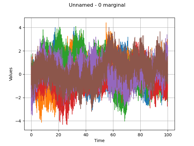
sample = process.getSample(6)
graph = sample.drawMarginal(0)
view = viewer.View(graph)
plt.show()

We notice here that we are able to sample the covariance model over a mesh of size 10000, which is usually tricky on laptop. This is mainly due to the compression.
Total running time of the script: ( 0 minutes 1.269 seconds)
 OpenTURNS