Draw fields

The objective here is to manipulate a multivariate stochastic process , where is discretized on the mesh and exhibit some of the services exposed by the Process objects:

• ask for the dimension, with the method getOutputDimension

• ask for the mesh, with the method getMesh

• ask for the mesh as regular 1-d mesh, with the getTimeGrid method

• ask for a realization, with the method the getRealization method

• ask for a continuous realization, with the getContinuousRealization method

• ask for a sample of realizations, with the getSample method

• ask for the normality of the process with the isNormal method

• ask for the stationarity of the process with the isStationary method

from __future__ import print_function
import openturns as ot
import openturns.viewer as viewer
from matplotlib import pylab as plt
import math as m
ot.Log.Show(ot.Log.NONE)

We create a mesh -a time grid- which is a RegularGrid :

tMin = 0.0
timeStep = 0.1
n = 100
time_grid = ot.RegularGrid(tMin, timeStep, n)
time_grid.setName('time')

We create a Normal process in dimension 3 with an exponential covariance model. We define the amplitude and the scale of the ExponentialModel

scale = [4.0]
amplitude = [1.0, 2.0, 3.0]

We define a spatial correlation :

spatialCorrelation = ot.CorrelationMatrix(3)
spatialCorrelation[0, 1] = 0.8
spatialCorrelation[0, 2] = 0.6
spatialCorrelation[1, 2] = 0.1

The covariance model is now created with :

myCovarianceModel = ot.ExponentialModel(scale, amplitude, spatialCorrelation)

Eventually, the process is built with :

process = ot.GaussianProcess(myCovarianceModel, time_grid)

The dimension d of the process may be retrieved by

dim = process.getOutputDimension()
print("Dimension : %d"%dim)

Out:

Dimension : 3

The underlying mesh of the process is obtained with the getMesh method :

mesh = process.getMesh()

We have access to peculiar data of the mesh such as the corners :

minMesh = mesh.getVertices().getMin()[0]
maxMesh = mesh.getVertices().getMax()[0]

We draw it :

graph = mesh.draw()
graph.setTitle("Time grid (mesh)")
graph.setXTitle("t")
graph.setYTitle("")
view = viewer.View(graph)

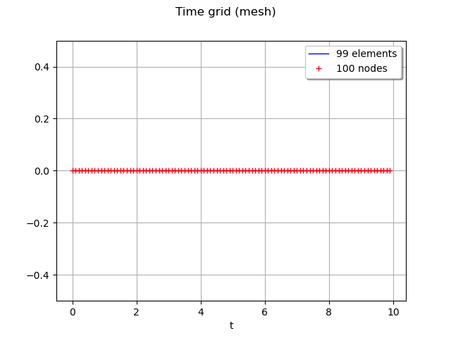
We can get the time grid of the process when the mesh can be interpreted as a regular time grid :

print( process.getTimeGrid() )

Out:

RegularGrid(start=0, step=0.1, n=100)

A typical feature of a process is the generation of a realization of itself :

realization = process.getRealization()

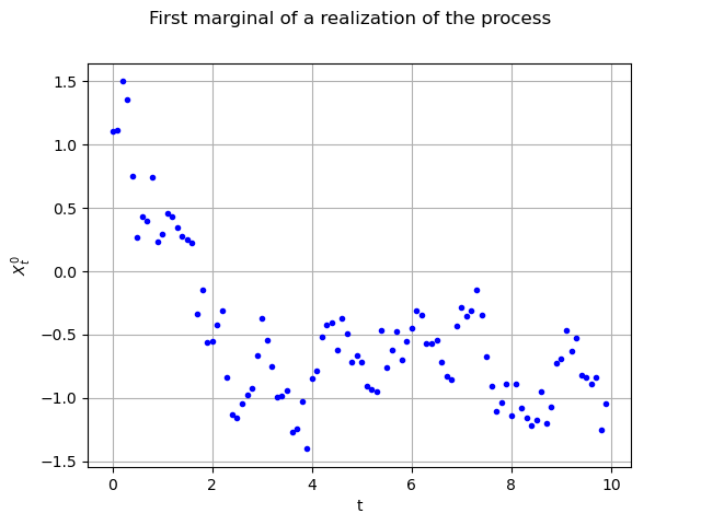
Here it is a sample of size (100 time steps, 3 spatial cooordinates and the time variable). We are able to draw its marginals, for instance the first (index 0) one , against the time with no interpolation :

interpolate=False
graph = realization.drawMarginal(0, interpolate)
graph.setTitle("First marginal of a realization of the process")
graph.setXTitle("t")
graph.setYTitle(r"$X_t^0$")
view = viewer.View(graph)

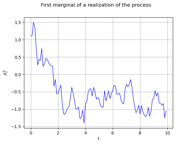
The same graph, but with interpolated values (default behaviour) :

graph = realization.drawMarginal(0)
graph.setTitle("First marginal of a realization of the process")
graph.setXTitle("t")
graph.setYTitle(r"$X_t^0$")
view = viewer.View(graph)

We can build a function representing the process using P1-Lagrange interpolation (when not defined from a functional model).

continuousRealization = process.getContinuousRealization()

Once again we draw its first marginal :

marginal0 = continuousRealization.getMarginal(0)
graph = marginal0.draw(minMesh, maxMesh)
graph.setTitle("First marginal of a P1-Lagrange continuous realization of the process")
graph.setXTitle("t")
view = viewer.View(graph)

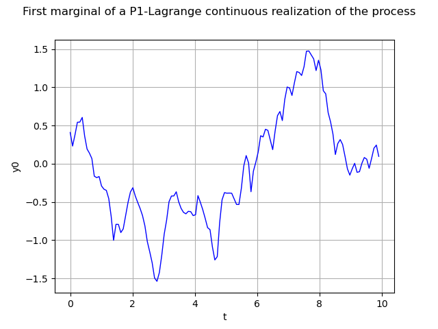
Please note that the marginal0 object is a function. Consequently we can evaluate it at any point of the domain, say

t0 = 3.5678
print(t0, marginal0([t0]))

Out:

3.5678 [-0.593188]

Several realizations of the process may be determined at once :

number = 10
fieldSample = process.getSample(number)

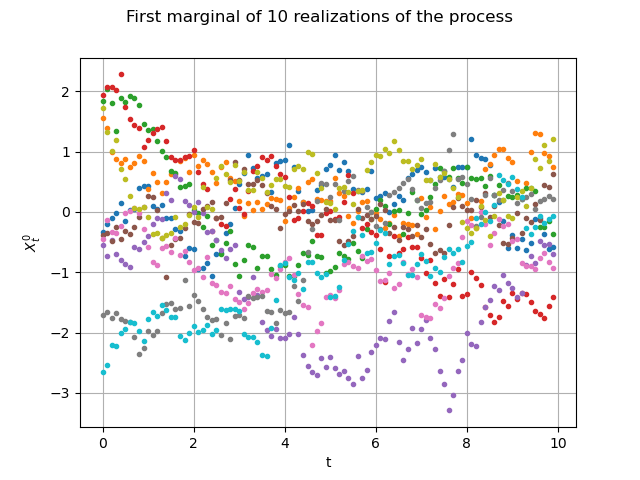
Let us draw them the first marginal)

graph = fieldSample.drawMarginal(0, False)
graph.setTitle("First marginal of 10 realizations of the process")
graph.setXTitle("t")
graph.setYTitle(r"$X_t^0$")
view = viewer.View(graph)

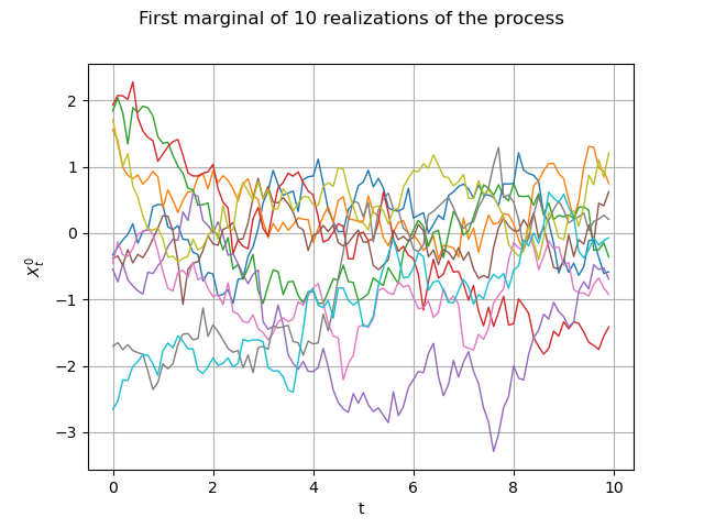
Same graph, but with interpolated values :

graph = fieldSample.drawMarginal(0)
graph.setTitle("First marginal of 10 realizations of the process")
graph.setXTitle("t")
graph.setYTitle(r"$X_t^0$")
view = viewer.View(graph)

Miscellanies

We can extract any marginal of the process with the getMarginal method. Beware the numerotation begins at 0 ! It may be not implemented yet for some processes. The extracted marginal is a 1D gaussian process :

print(process.getMarginal([1]))

Out:

GaussianProcess(trend=[x0]->[0.0], covariance=ExponentialModel(scale=[4], amplitude=[2], no spatial correlation))

If we extract simultaneously two indices we build a 2D gaussian process :

print(process.getMarginal([0, 2]))

Out:

GaussianProcess(trend=[x0]->[0.0,0.0], covariance=ExponentialModel(scale=[4], amplitude=[1,3], spatial correlation=
[[ 1   0.6 ]
 [ 0.6 1   ]]))

We can check whether the process is normal or not :

print( "Is normal ? ", process.isNormal() )

Out:

Is normal ?  True

and the stationarity as well :

print( "Is stationary ? ", process.isStationary() )

plt.show()

Out:

Is stationary ?  True