Note
Click here to download the full example code
Create a stationary covariance model
This use case illustrates how the user can define his own stationary covariance model thanks to the object UserDefinedStationaryCovarianceModel defined from:
a mesh
of dimension
defined by the vertices
and the associated simplices,
a collection of covariance matrices stored in the object CovarianceMatrixCollection noted
where
for
Then we build a stationary covariance function which is a piecewise constant function on defined by:
where is such that
is the vertex of
the nearest to
from __future__ import print_function
import openturns as ot
import openturns.viewer as viewer
from matplotlib import pylab as plt
ot.Log.Show(ot.Log.NONE)
We detail the example described in the documentation Create the time grid
t0 = 0.0
dt = 0.5
N = int((20.0 - t0) / dt)
mesh = ot.RegularGrid(t0, dt, N)

# Create the covariance function


def gamma(tau):
    return 1.0 / (1.0 + tau * tau)

# Create the collection of HermitianMatrix
coll = ot.SquareMatrixCollection()
for k in range(N):
    t = mesh.getValue(k)
    matrix = ot.SquareMatrix([[gamma(t)]])
    coll.add(matrix)
Create the covariance model
covmodel = ot.UserDefinedStationaryCovarianceModel(mesh, coll)

# One vertex of the mesh
tau = 1.5

# Get the covariance function computed at the vertex tau
covmodel(tau)
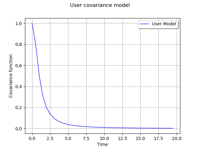
Graph of the spectral function
x = ot.Sample(N, 2)
for k in range(N):
    t = mesh.getValue(k)
    x[k, 0] = t
    value = covmodel(t)
    x[k, 1] = value[0, 0]

# Create the curve of the spectral function
curve = ot.Curve(x, 'User Model')

# Create the graph
myGraph = ot.Graph('User covariance model', 'Time', 'Covariance function', True)
myGraph.add(curve)
myGraph.setLegendPosition('topright')
view = viewer.View(myGraph)
plt.show()

Total running time of the script: ( 0 minutes 0.111 seconds)
 OpenTURNS