Calibration of the logistic model

We present a calibration study of the logistic growth model defined here.

Analysis of the data

from openturns.usecases import logistic_model as logistic_model
import openturns as ot
import numpy as np
import openturns.viewer as viewer
from matplotlib import pylab as plt
ot.Log.Show(ot.Log.NONE)

We load the logistic model from the usecases module :

lm = logistic_model.LogisticModel()

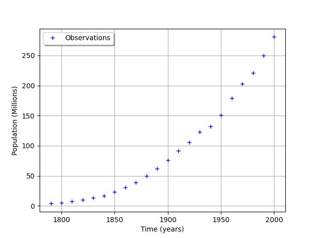
The data is based on 22 dates from 1790 to 2000. The observation points are stored in the data field :

observedSample = lm.data

nbobs = observedSample.getSize()
nbobs

Out:

22

timeObservations = observedSample[:, 0]
timeObservations[0:5]

	v0
0	1790
1	1800
2	1810
3	1820
4	1830

populationObservations = observedSample[:, 1]
populationObservations[0:5]

	v1
0	3.9
1	5.3
2	7.2
3	9.6
4	13

graph = ot.Graph('', 'Time (years)', 'Population (Millions)', True, 'topleft')
cloud = ot.Cloud(timeObservations, populationObservations)
cloud.setLegend("Observations")
graph.add(cloud)
view = viewer.View(graph)

We consider the times and populations as dimension 22 vectors. The logisticModel function takes a dimension 24 vector as input and returns a dimension 22 vector. The first 22 components of the input vector contains the dates and the remaining 2 components are and .

nbdates = 22


def logisticModel(X):
    t = [X[i] for i in range(nbdates)]
    a = X[22]
    c = X[23]
    t0 = 1790.
    y0 = 3.9e6
    b = np.exp(c)
    y = [0.0] * nbdates
    for i in range(nbdates):
        y[i] = a*y0/(b*y0+(a-b*y0)*np.exp(-a*(t[i]-t0)))
    z = [yi/1.e6 for yi in y]  # Convert into millions
    return z

logisticModelPy = ot.PythonFunction(24, nbdates, logisticModel)

The reference values of the parameters.

Because is so small with respect to , we use the logarithm.

np.log(1.5587e-10)

Out:

-22.581998789427587

a = 0.03134
c = -22.58
thetaPrior = [a, c]

logisticParametric = ot.ParametricFunction(
    logisticModelPy, [22, 23], thetaPrior)

Check that we can evaluate the parametric function.

populationPredicted = logisticParametric(timeObservations.asPoint())
populationPredicted

[3.9,5.29757,7.17769,9.69198,13.0277,17.4068,23.0769,30.2887,39.2561,50.0977,62.7691,77.0063,92.311,108.001,123.322,137.59,150.3,161.184,170.193,177.442,183.144,187.55]#22

graph = ot.Graph('', 'Time (years)', 'Population (Millions)', True, 'topleft')
# Observations
cloud = ot.Cloud(timeObservations, populationObservations)
cloud.setLegend("Observations")
cloud.setColor("blue")
graph.add(cloud)
# Predictions
cloud = ot.Cloud(timeObservations.asPoint(), populationPredicted)
cloud.setLegend("Predictions")
cloud.setColor("green")
graph.add(cloud)
view = viewer.View(graph)

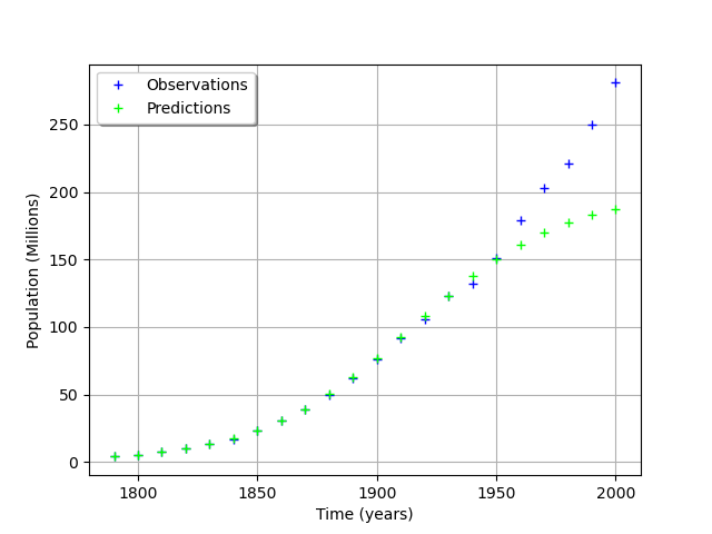
We see that the fit is not good: the observations continue to grow after 1950, while the growth of the prediction seem to fade.

Calibration with linear least squares

timeObservationsVector = ot.Sample(
    [[timeObservations[i, 0] for i in range(nbobs)]])
timeObservationsVector[0:10]

	v0	v1	v2	v3	v4	v5	v6	v7	v8	v9	v10	v11	v12	v13	v14	v15	v16	v17	v18	v19	v20	v21
0	1790	1800	1810	1820	1830	1840	1850	1860	1870	1880	1890	1900	1910	1920	1930	1940	1950	1960	1970	1980	1990	2000

populationObservationsVector = ot.Sample(
    [[populationObservations[i, 0] for i in range(nbobs)]])
populationObservationsVector[0:10]

	v0	v1	v2	v3	v4	v5	v6	v7	v8	v9	v10	v11	v12	v13	v14	v15	v16	v17	v18	v19	v20	v21
0	3.9	5.3	7.2	9.6	13	17	23	31	39	50	62	76	92	106	123	132	151	179	203	221	250	281

The reference values of the parameters.

a = 0.03134
c = -22.58
thetaPrior = [a, c]

logisticParametric = ot.ParametricFunction(
    logisticModelPy, [22, 23], thetaPrior)

Check that we can evaluate the parametric function.

populationPredicted = logisticParametric(timeObservationsVector)
populationPredicted[0:10]

	y0	y1	y2	y3	y4	y5	y6	y7	y8	y9	y10	y11	y12	y13	y14	y15	y16	y17	y18	y19	y20	y21
0	3.9	5.297571	7.177694	9.691977	13.02769	17.40682	23.07691	30.2887	39.25606	50.09767	62.76907	77.0063	92.31103	108.0009	123.3223	137.5899	150.3003	161.1843	170.193	177.4422	183.1443	187.5496

Calibration

algo = ot.LinearLeastSquaresCalibration(
    logisticParametric, timeObservationsVector, populationObservationsVector, thetaPrior)

algo.run()

calibrationResult = algo.getResult()

thetaMAP = calibrationResult.getParameterMAP()
thetaMAP

[0.0265958,-23.1714]

thetaPosterior = calibrationResult.getParameterPosterior()
thetaPosterior.computeBilateralConfidenceIntervalWithMarginalProbability(0.95)[
    0]

[0.0246465, 0.028545]
[-23.3182, -23.0247]

transpose samples to interpret several observations instead of several input/outputs as it is a field model

if calibrationResult.getInputObservations().getSize() == 1:
    calibrationResult.setInputObservations(
        [timeObservations[i] for i in range(nbdates)])
    calibrationResult.setOutputObservations(
        [populationObservations[i] for i in range(nbdates)])
    outputAtPrior = [[calibrationResult.getOutputAtPriorMean()[0, i]]
                     for i in range(nbdates)]
    outputAtPosterior = [
        [calibrationResult.getOutputAtPosteriorMean()[0, i]] for i in range(nbdates)]
    calibrationResult.setOutputAtPriorAndPosteriorMean(
        outputAtPrior, outputAtPosterior)

graph = calibrationResult.drawObservationsVsInputs()
view = viewer.View(graph)

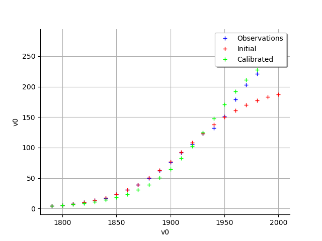
graph = calibrationResult.drawObservationsVsInputs()
view = viewer.View(graph)

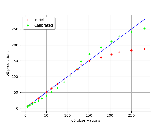
graph = calibrationResult.drawObservationsVsPredictions()
view = viewer.View(graph)

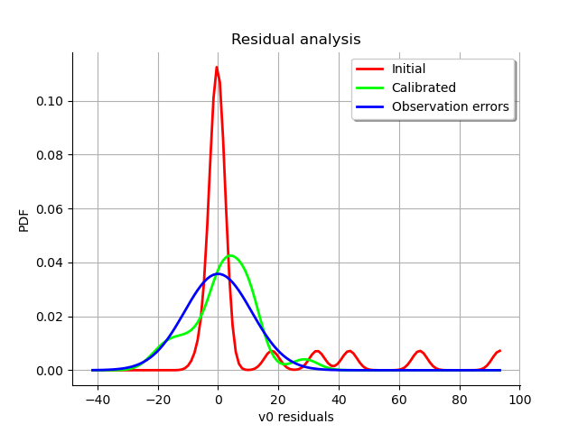
graph = calibrationResult.drawResiduals()
view = viewer.View(graph)

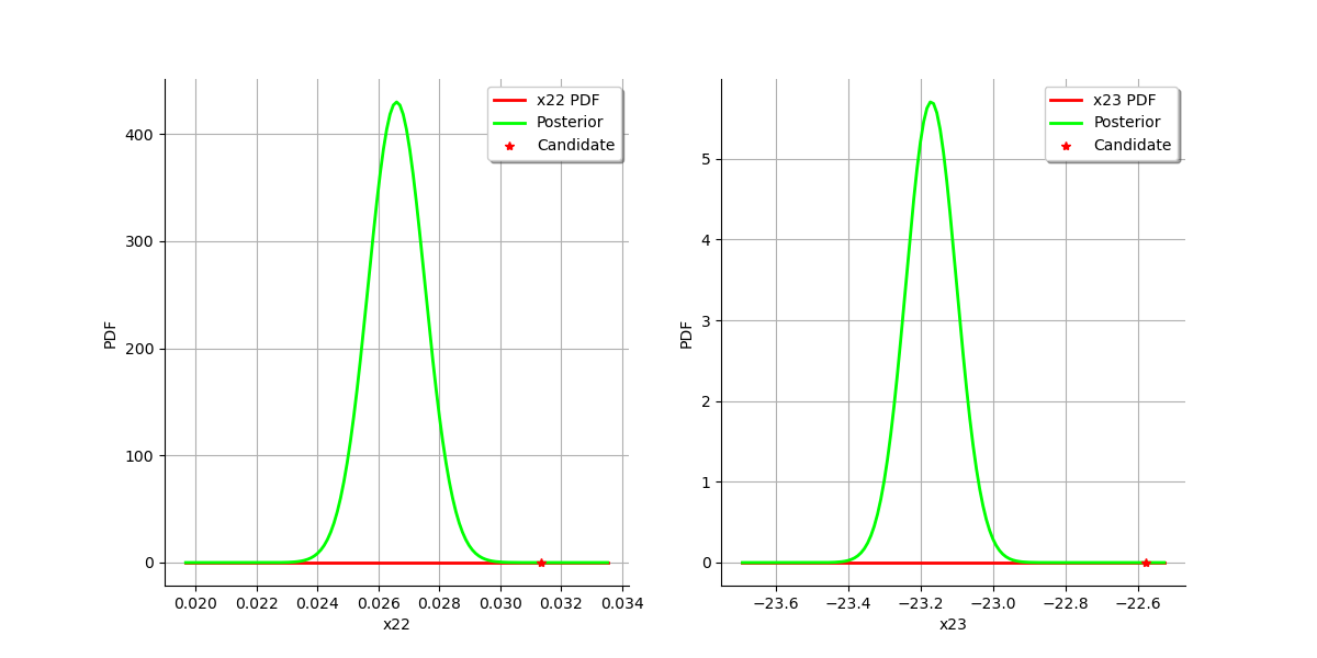
graph = calibrationResult.drawParameterDistributions()
view = viewer.View(graph)

plt.show()