Estimate a conditional quantile

# sphinx_gallery_thumbnail_number = 8

From a multivariate data sample we estimate its distribution with kernel smoothing. Here we present a bivariate distribution X= (X1, X2). We use the computeConditionalQuantile method to estimate the 90% quantile of the conditional variable :

We then draw the curve . We first start with independent normals then we consider dependent marginals with a Clayton copula.

from __future__ import print_function
import openturns as ot
import openturns.viewer as viewer
from matplotlib import pylab as plt
import numpy as np
ot.Log.Show(ot.Log.NONE)

Set the random generator seed

ot.RandomGenerator.SetSeed(0)

Defining the marginals

We consider two independent normal marginals :

X1 = ot.Normal(0.0, 1.0)
X2 = ot.Normal(0.0, 3.0)

Independent marginals

distX = ot.ComposedDistribution([X1, X2])
sample = distX.getSample(1000)

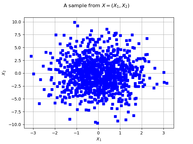
Let’s see the data

graph = ot.Graph('2D-Normal sample', 'x1', 'x2', True, '')
cloud = ot.Cloud(sample, 'blue', 'fsquare', 'My Cloud')
graph.add(cloud)
graph.setXTitle("$X_1$")
graph.setYTitle("$X_2$")
graph.setTitle("A sample from $X=(X_1, X_2)$")
view = viewer.View(graph)

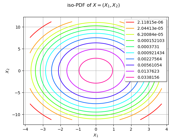
We draw the isolines of the PDF of :

graph = distX.drawPDF()
graph.setXTitle("$X_1$")
graph.setYTitle("$X_2$")
graph.setTitle("iso-PDF of $X=(X_1, X_2)$")
view = viewer.View(graph)

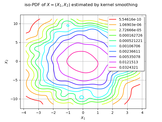
We estimate the density with kernel smoothing :

kernel = ot.KernelSmoothing()
estimated = kernel.build(sample)

We draw the isolines of the estimated PDF of :

graph = estimated.drawPDF()
graph.setXTitle("$X_1$")
graph.setYTitle("$X_2$")
graph.setTitle("iso-PDF of $X=(X_1, X_2)$ estimated by kernel smoothing")
view = viewer.View(graph)

We can compute the conditional quantile of with the computeConditionalQuantile method and draw it after.

We first create N observation points in :

N = 301
xobs = np.linspace(-3.0, 3.0, N)
sampleObs = ot.Sample([[xi] for xi in xobs])

We create curves of the exact and approximated quantile

x = [xi for xi in xobs]
yapp = [estimated.computeConditionalQuantile(
    0.9, sampleObs[i]) for i in range(N)]
yex = [distX.computeConditionalQuantile(0.9, sampleObs[i]) for i in range(N)]

cxy_app = ot.Curve(x, yapp)
cxy_ex = ot.Curve(x, yex)
graph = ot.Graph('90% quantile of $X_1 | X_2=x_2$',
                 '$x_2$', '$Q_1(x_2)$', True, '')
graph.add(cxy_app)
graph.add(cxy_ex)
graph.setLegends(["$Q_1$ kernel smoothing", "$Q_1$ exact"])
graph.setLegendPosition('bottomright')
graph.setColors(["red", "blue"])
view = viewer.View(graph)

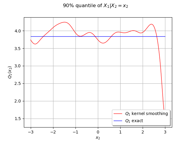
In this case the Q_1 quantile is constant because of the independance of the marginals.

Dependance through a Clayton copula

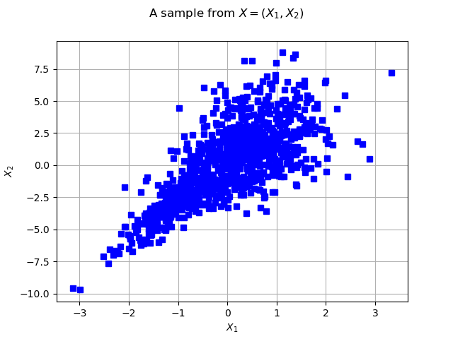
We now define a Clayton copula to model the dependance between our marginals. The Clayton copula is a bivariate asymmmetric Archimedean copula, exhibiting greater dependence in the negative tail than in the positive.

copula = ot.ClaytonCopula(2.5)
distX = ot.ComposedDistribution([X1, X2], copula)

We generate a sample from the distribution :

sample = distX.getSample(1000)

Let’s see the data

graph = ot.Graph('2D-Normal sample', 'x1', 'x2', True, '')
cloud = ot.Cloud(sample, 'blue', 'fsquare', 'My Cloud')
graph.add(cloud)
graph.setXTitle("$X_1$")
graph.setYTitle("$X_2$")
graph.setTitle("A sample from $X=(X_1, X_2)$")
view = viewer.View(graph)

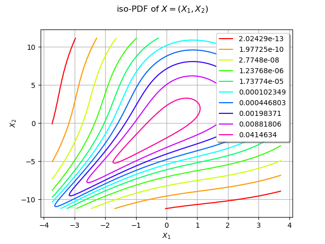
We draw the isolines of the PDF of :

graph = distX.drawPDF()
graph.setXTitle("$X_1$")
graph.setYTitle("$X_2$")
graph.setTitle("iso-PDF of $X=(X_1, X_2)$")
view = viewer.View(graph)

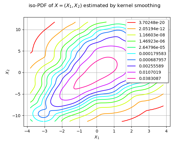
We estimate the density with kernel smoothing :

kernel = ot.KernelSmoothing()
estimated = kernel.build(sample)

We draw the isolines of the estimated PDF of :

graph = estimated.drawPDF()
graph.setXTitle("$X_1$")
graph.setYTitle("$X_2$")
graph.setTitle("iso-PDF of $X=(X_1, X_2)$ estimated by kernel smoothing")
view = viewer.View(graph)

We can compute the conditional quantile of with the computeConditionalQuantile method and draw it after.

We first create N observation points in :

N = 301
xobs = np.linspace(-3.0, 3.0, N)
sampleObs = ot.Sample([[xi] for xi in xobs])

We create curves of the exact and approximated quantile

x = [xi for xi in xobs]
yapp = [estimated.computeConditionalQuantile(
    0.9, sampleObs[i]) for i in range(N)]
yex = [distX.computeConditionalQuantile(0.9, sampleObs[i]) for i in range(N)]

cxy_app = ot.Curve(x, yapp)
cxy_ex = ot.Curve(x, yex)
graph = ot.Graph('90% quantile of $X_1 | X_2=x_2$',
                 '$x_2$', '$Q_1(x_2)$', True, '')
graph.add(cxy_app)
graph.add(cxy_ex)
graph.setLegends(["$Q_1$ kernel smoothing", "$Q_1$ exact"])
graph.setLegendPosition('bottomright')
graph.setColors(["red", "blue"])
view = viewer.View(graph)

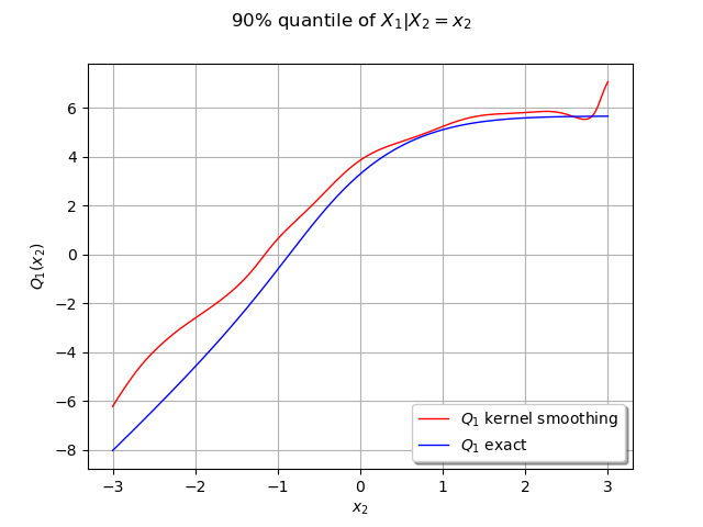
Our estimated conditional quantile is a good approximate and should be better the more data we have. We can observe it by increasing the number of samples.

plt.show()