Logistic growth model

In this example, we use the logistic growth model in order to show how to define a function which has a vector input and a field output. We use the OpenTURNSPythonPointToFieldFunction class to define the derived class and its methods.

Define the model

from __future__ import print_function
from openturns.usecases import logistic_model as logistic_model
import openturns as ot
import openturns.viewer as viewer
from matplotlib import pylab as plt
from numpy import linspace, exp, maximum
ot.Log.Show(ot.Log.NONE)

We load the logistic model from the usecases module :

lm = logistic_model.LogisticModel()

We get the data from the LogisticModel data class (22 dates with population) :

ustime = lm.data.getMarginal(0)
uspop = lm.data.getMarginal(1)

We get the input parameters distribution distX :

distX = lm.distX

We define the model :

class Popu(ot.OpenTURNSPythonPointToFieldFunction):

    def __init__(self, t0=1790.0, tfinal=2000.0, nt=1000):
        grid = ot.RegularGrid(t0, (tfinal - t0) / (nt - 1), nt)
        super(Popu, self).__init__(3, grid, 1)
        self.setInputDescription(['y0', 'a', 'b'])
        self.setOutputDescription(['N'])
        self.ticks_ = [t[0] for t in grid.getVertices()]
        self.phi_ = ot.SymbolicFunction(['t', 'y', 'a', 'b'], ['a*y - b*y^2'])

    def _exec(self, X):
        y0 = X[0]
        a = X[1]
        b = X[2]
        phi_ab = ot.ParametricFunction(self.phi_, [2, 3], [a, b])
        phi_t = ot.ParametricFunction(phi_ab, [0], [0.0])
        solver = ot.RungeKutta(phi_t)
        initialState = [y0]
        values = solver.solve(initialState, self.ticks_)
        return values * [1.0e-6]


F = Popu(1790.0, 2000.0, 1000)
popu = ot.PointToFieldFunction(F)

Generate a sample from the model

Sample from the model

size = 10
inputSample = distX.getSample(size)
outputSample = popu(inputSample)

ot.ResourceMap.SetAsUnsignedInteger('Drawable-DefaultPalettePhase', size)

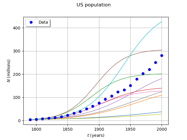
Draw some curves

graph = outputSample.drawMarginal(0)
graph.setTitle('US population')
graph.setXTitle(r'$t$ (years)')
graph.setYTitle(r'$N$ (millions)')
cloud = ot.Cloud(ustime, uspop)
cloud.setPointStyle('circle')
cloud.setLegend('Data')
graph.add(cloud)
graph.setLegendPosition('topleft')
view = viewer.View(graph)
plt.show()