Note

Click here to download the full example code

Kriging : choose a trend vector space¶

import openturns as ot
import openturns.viewer as otv
from matplotlib import pylab as plt

Introduction¶

In this example we present the basic trends which we may use in the kriging metamodel procedure :

ConstantBasis ;

LinearBasis ;

QuadraticBasis ;

The model is the simple real function defined by

$f : x \mapsto x \left( \sin \frac{x}{2} \right)$

which we study on the $[0,10]$ interval.

dimension = 1

The focus being on the trend we assume a given squared exponential covariance kernel :

$C_{\theta}(s,t) = \sigma^2 e^{ - \frac{(t-s)^2}{2\rho^2} }$

where $\theta = (\sigma, \rho)$ is the hyperparameters vectors. The nature of the covariance model is fixed but its parameters are calibrated during the kriging process. We want to choose them so as to best fit our data.

Eventually the kriging (meta)model $\hat{Y}(x)$ reads as

$\hat{Y}(x) = m(x) + Z(x)$

where $m(.)$ is the trend and $Z(.)$ is a gaussian process with zero-mean and its covariance matrix is $C_{\theta}(s,t)$ . The trend is deterministic and the gaussian process is probabilistc but they both contribute to the metamodel. A special feature of the kriging is the interpolation property : the metamodel is exact at the trainig data.

covarianceModel = ot.SquaredExponential([1.], [1.0])

We define our exact model with a SymbolicFunction :

model = ot.SymbolicFunction(['x'], ['x*sin(0.5*x)'])

We use the following sample to train our metamodel :

nTrain = 5
Xtrain = ot.Sample([[0.5], [1.3], [2.4], [5.6], [8.9]])

The values of the exact model are also needed for training :

Ytrain = model(Xtrain)

We shall test the model on a set of points and use a regular grid for this matter.

nTest = 101
step = 0.1
x_test = ot.RegularGrid(0, step, nTest).getVertices()

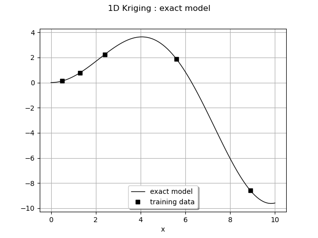
We draw the training points and the model at the testing points. We encapsulate it into a function to use it again later.

def plot_exact_model():
    graph = ot.Graph('', 'x', '', True, '')
    y_test = model(x_test)
    curveModel = ot.Curve(x_test, y_test)
    curveModel.setLineStyle("solid")
    curveModel.setColor("black")
    graph.add(curveModel)
    cloud = ot.Cloud(Xtrain, Ytrain)
    cloud.setColor("black")
    cloud.setPointStyle("fsquare")
    graph.add(cloud)
    return graph

graph = plot_exact_model()
graph.setLegends(['exact model', 'training data'])
graph.setLegendPosition("bottom")
graph.setTitle('1D Kriging : exact model')
view = otv.View(graph)

A common pre-processing step is to apply a transform on the input data before performing the kriging. To do so we write a linear transform of our input data : we make it unit centered at its mean. Then we fix the mean and the standard deviation to their values with the ParametricFunction. We build the inverse transform as well.

We first compute the mean and standard deviation of the input data :

mean = Xtrain.computeMean()[0]
stdDev = Xtrain.computeStandardDeviation()[0]
print("Xtrain, mean : %.3f" % mean)
print("Xtrain, standard deviation : %.3f" % stdDev)

Out:

Xtrain, mean : 3.740
Xtrain, standard deviation : 3.476

tf = ot.SymbolicFunction(['mu', 'sigma', 'x'], ['(x-mu)/sigma'])
itf = ot.SymbolicFunction(['mu', 'sigma', 'x'], ['sigma*x+mu'])
myInverseTransform = ot.ParametricFunction(itf, [0, 1], [mean, stdDev])
myTransform = ot.ParametricFunction(tf, [0, 1], [mean, stdDev])

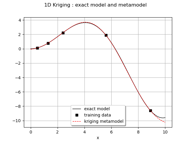
A constant basis¶

In this paragraph we choose a basis constant for the kriging. There is only one unknown which is the value of the constant. The basis is built with the ConstantBasisFactory class.

basis = ot.ConstantBasisFactory(dimension).build()

We build the kriging algorithm by giving it the transformed data, the output data, the covariance model and the basis.

algo = ot.KrigingAlgorithm(myTransform(Xtrain), Ytrain, covarianceModel, basis)

We can run the algorithm and store the result :

algo.run()
result = algo.getResult()

The metamodel is the following ComposedFunction :

metamodel = ot.ComposedFunction(result.getMetaModel(), myTransform)

We can draw the metamodel and the exact model on the same graph.

graph = plot_exact_model()
y_test = metamodel(x_test)
curve = ot.Curve(x_test, y_test)
curve.setLineStyle("dashed")
curve.setColor("red")
graph.add(curve)
graph.setLegends(['exact model', 'training data', 'kriging metamodel'])
graph.setLegendPosition("bottom")
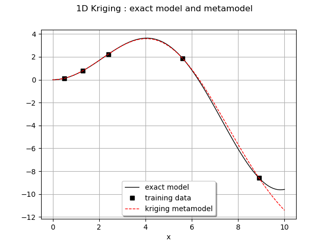
graph.setTitle('1D Kriging : exact model and metamodel')
view = otv.View(graph)

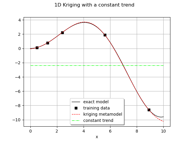
We can retrieve the calibrated trend coefficient :

c0 = result.getTrendCoefficients()
print("The trend is the curve m(x) = %.6e" % c0[0][0])

Out:

The trend is the curve m(x) = -2.393406e+00

We also pay attention to the trained covariance model and observe the values of the hyperparameters :

rho = result.getCovarianceModel().getScale()[0]
print("Scale parameter : %.3e" % rho)

sigma = result.getCovarianceModel().getAmplitude()[0]
print("Amplitude parameter : %.3e" % sigma)

Out:

Scale parameter : 9.428e-01
Amplitude parameter : 6.305e+00

We build the trend from the coefficient :

constantTrend = ot.SymbolicFunction(['a', 'x'], ['a'])
myTrend = ot.ParametricFunction(constantTrend, [0], [c0[0][0]])

We draw the trend found by the kriging procedure :

y_test = myTrend(myTransform(x_test))
curve = ot.Curve(x_test, y_test)
curve.setLineStyle("dotdash")
curve.setColor("green")
graph.add(curve)
graph.setLegends(['exact model', 'training data',
                  'kriging metamodel', 'constant trend'])
graph.setLegendPosition("bottom")
graph.setTitle('1D Kriging with a constant trend')
view = otv.View(graph)

We create a small function returning bounds of the 68% confidence interval $[-sigma,sigma]$ :

def plot_ICBounds(x_test, y_test, nTest, sigma):
    vUp = [[x_test[i][0], y_test[i][0] + sigma] for i in range(nTest)]
    vLow = [[x_test[i][0], y_test[i][0] - sigma] for i in range(nTest)]
    polyData = [[vLow[i], vLow[i+1], vUp[i+1], vUp[i]] for i in range(nTest-1)]
    polygonList = [ot.Polygon(polyData[i], "grey", "grey")
                   for i in range(nTest-1)]
    boundsPoly = ot.PolygonArray(polygonList)
    return boundsPoly

We now draw it :

boundsPoly = plot_ICBounds(x_test, y_test, nTest, sigma)
graph.add(boundsPoly)
graph.setLegends(['exact model', 'training data', 'kriging metamodel',
                  'constant trend', '68% - confidence interval'])
graph.setLegendPosition("bottom")
graph.setTitle('1D Kriging with a constant trend')
view = otv.View(graph)

As expected with a constant basis, the trend obtained is an horizontal line amidst data points. The main idea is that at any point $x_0$ , the gaussian term $Z(x_0)$ helps to find a good value of $\hat{Y}(x_0)$ thanks to the high value of the amplitude $\sigma$ ( $\sigma \approx 6.359$ ) far away from the mean $m(x)$ . As a consequence the 68% confidence interval is wide.

Linear basis¶

With a linear basis, the vector space is defined by the basis $\{1, X\}$ : that is all the lines of the form $y(X) = aX + b$ .

basis = ot.LinearBasisFactory(dimension).build()

We run the kriging analysis and store the result :

algo = ot.KrigingAlgorithm(myTransform(Xtrain), Ytrain, covarianceModel, basis)
algo.run()
result = algo.getResult()
metamodel = ot.ComposedFunction(result.getMetaModel(), myTransform)

We can draw the metamodel and the exact model on the same graph.

graph = plot_exact_model()
y_test = metamodel(x_test)
curve = ot.Curve(x_test, y_test)
curve.setLineStyle("dashed")
curve.setColor("red")
graph.add(curve)
graph.setLegends(['exact model', 'training data', 'kriging metamodel'])
graph.setLegendPosition("bottom")
graph.setTitle('1D Kriging : exact model and metamodel')
view = otv.View(graph)

We can retrieve the calibrated trend coefficients with getTrendCoefficients :

c0 = result.getTrendCoefficients()
print("Trend is the curve m(X) = %.6e X + %.6e" % (c0[0][1], c0[0][0]))

Out:

Trend is the curve m(X) = -4.065459e+00 X + -1.937932e+00

We also pay attention to the trained covariance model and observe the values of the hyperparameters :

rho = result.getCovarianceModel().getScale()[0]
print("Scale parameter : %.3e" % rho)

sigma = result.getCovarianceModel().getAmplitude()[0]
print("Amplitude parameter : %.3e" % sigma)

Out:

Scale parameter : 9.443e-01
Amplitude parameter : 5.513e+00

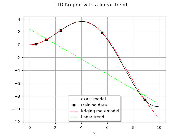
We draw the linear trend that we are interested in.

linearTrend = ot.SymbolicFunction(['a', 'b', 'x'], ['a*x+b'])
myTrend = ot.ParametricFunction(linearTrend, [0, 1], [c0[0][1], c0[0][0]])
y_test = myTrend(myTransform(x_test))
curve = ot.Curve(x_test, y_test)
curve.setLineStyle("dotdash")
curve.setColor("green")
graph.add(curve)
graph.setLegends(['exact model', 'training data',
                  'kriging metamodel', 'linear trend'])
graph.setLegendPosition("bottom")
graph.setTitle('1D Kriging with a linear trend')
view = otv.View(graph)

The same graphic with the 68% confidence interval :

boundsPoly = plot_ICBounds(x_test, y_test, nTest, sigma)
graph.add(boundsPoly)
graph.setLegends(['exact model', 'training data', 'kriging metamodel',
                  'linear trend', '68% - confidence interval'])
graph.setLegendPosition("bottom")
graph.setTitle('1D Kriging with a linear trend')
view = otv.View(graph)

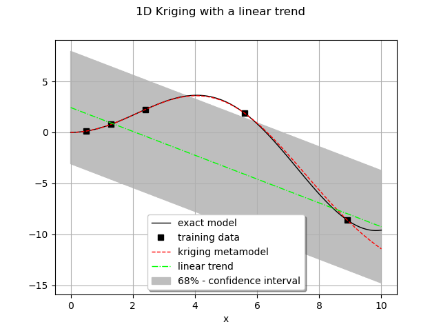
The trend obtained is decreasing on the interval of study : that is the general trend we observe from the exact model. It is still nowhere close to the exact model but as in the constant case the gaussian part will do the job of building a correct (visually at least) metamodel. We note that the values of the amplitude and the scale parameters are similar to the previous constant case. As it can be seen on the previous figure the metamodel is interpolating (see the last data point).

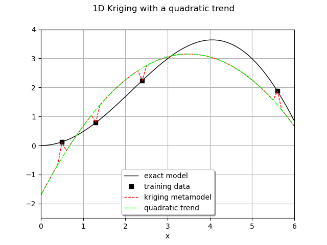
Quadratic basis¶

In this last paragraph we turn to the quadratic basis. All subsequent analysis should remain the same.

basis = ot.QuadraticBasisFactory(dimension).build()

We run the kriging analysis and store the result :

algo = ot.KrigingAlgorithm(myTransform(Xtrain), Ytrain, covarianceModel, basis)
algo.run()
result = algo.getResult()
metamodel = ot.ComposedFunction(result.getMetaModel(), myTransform)

We can draw the metamodel and the exact model on the same graph.

graph = plot_exact_model()
y_test = metamodel(x_test)
curve = ot.Curve(x_test, y_test)
curve.setLineStyle("dashed")
curve.setColor("red")
graph.add(curve)
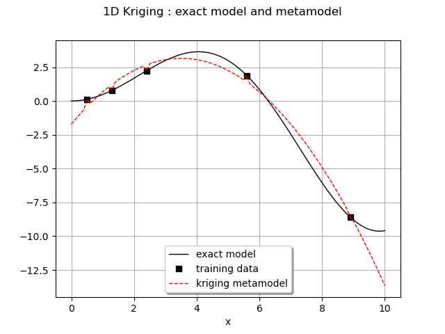
graph.setLegends(['exact model', 'training data', 'kriging metamodel'])
graph.setLegendPosition("bottom")
graph.setTitle('1D Kriging : exact model and metamodel')
view = otv.View(graph)

We can retrieve the calibrated trend coefficients with getTrendCoefficients :

c0 = result.getTrendCoefficients()
print("Trend is the curve m(X) = %.6e X**2 + %.6e X + %.6e" %
      (c0[0][2], c0[0][1], c0[0][0]))

Out:

Trend is the curve m(X) = -4.804137e+00 X**2 + -6.654850e-01 X + 3.128888e+00

We also pay attention to the trained covariance model and observe the values of the hyperparameters :

rho = result.getCovarianceModel().getScale()[0]
print("Scale parameter : %.3e" % rho)

sigma = result.getCovarianceModel().getAmplitude()[0]
print("Amplitude parameter : %.3e" % sigma)

Out:

Scale parameter : 1.000e-02
Amplitude parameter : 6.844e-01

The quadratic linear trend obtained is :

quadraticTrend = ot.SymbolicFunction(['a', 'b', 'c', 'x'], ['a*x^2 + b*x + c'])
myTrend = ot.ParametricFunction(quadraticTrend, [0, 1, 2], [
                                c0[0][2], c0[0][1], c0[0][0]])

In this case we restrict ourselves to the $[0,6] \times [-2.5,4]$ for visualization.

y_test = myTrend(myTransform(x_test))
curve = ot.Curve(x_test, y_test)
curve.setLineStyle("dotdash")
curve.setColor("green")
graph.add(curve)
graph.setLegends(['exact model', 'training data',
                  'kriging metamodel', 'quadratic trend'])
graph.setLegendPosition("bottom")
graph.setTitle('1D Kriging with a quadratic trend')
view = otv.View(graph)
axes = view.getAxes()
_ = axes[0].set_xlim(0.0, 6.0)
_ = axes[0].set_ylim(-2.5, 4.0)

sphinx_gallery_thumbnail_number = 10 The same graphic with the 68% confidence interval.

boundsPoly = plot_ICBounds(x_test, y_test, nTest, sigma)
graph.add(boundsPoly)
graph.setLegends(['exact model', 'training data', 'kriging metamodel',
                  'quadratic trend', '68% - confidence interval'])
graph.setLegendPosition("bottom")
graph.setTitle('1D Kriging with a quadratic trend')
view = otv.View(graph)
axes = view.getAxes()
_ = axes[0].set_xlim(0.0, 6.0)
_ = axes[0].set_ylim(-2.5, 4.0)

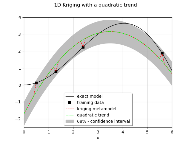
In this case the analysis is interesting to understand the general behaviour of the kriging process.

From the previous figure we feel that the metamodel is mostly characterized by the trend which is a good approximate of the exact solution over the interval. However, to a certain extent, we have lost flexibility by having a too good and rigid trend as we still have to impose the interpolation property.

We see that the gap between the trend and the exact model is small and the amplitude of the gaussian process is small as well : $\sigma \approx 0.684$ . Then the confidence interval is more narrow than before. The scale parameter is small, $\rho \approx 0.010$ , meaning that two distant points are rapidly independent. The only way to set the interpolation property is to create small peaks (see the figure). The sad conclusion is that the metamodel loses its smoothness.

In that case one should use a constant or linear basis even if a quadratic trend seems right.

Display figures

plt.show()

Total running time of the script: ( 0 minutes 1.360 seconds)

Gallery generated by Sphinx-Gallery

OpenTURNS

An Open source initiative for the Treatment of Uncertainties, Risks'N Statistics

Table of Contents

Previous topic

Next topic

This Page

Kriging : choose a trend vector space¶

Introduction¶

A constant basis¶

Linear basis¶

Quadratic basis¶