Kriging : propagate uncertainties

import openturns as ot
import numpy as np
from matplotlib import pylab as plt
import openturns.viewer as otv

In this example we propagate uncertainties through a kriging metamodel of the

Ishigami model.

We first build the metamodel and then compute its mean with a MonteCarlo computation.

We first load the Ishigami model from the usecases module :

from openturns.usecases import ishigami_function as ishigami_function
im = ishigami_function.IshigamiModel()

We build a design of experiments with a LHS for the three input variables supposed independent.

experiment = ot.LHSExperiment(im.distributionX, 30, False, True)
xdata = experiment.generate()

We get the exact model and evaluate it at the input training data xdata to build the output data ydata.

model = im.model
ydata = model(xdata)

We define our kriging strategy :

• a constant basis in ;

• a squared exponential covariance function.

dimension = 3
basis = ot.ConstantBasisFactory(dimension).build()
covarianceModel = ot.SquaredExponential([0.1]*dimension, [1.0])
algo = ot.KrigingAlgorithm(xdata, ydata, covarianceModel, basis)
algo.run()
result = algo.getResult()

We finally get the metamodel to use with MonteCarlo.

metamodel = result.getMetaModel()

We want to estmate the mean of the Ishigami model with MonteCarlo using the metamodel instead of the exact model.

We first create a random vector following the input distribution :

X = ot.RandomVector(im.distributionX)

And then we create a random vector from the image of the input random vector by the metamodel :

Y = ot.CompositeRandomVector(metamodel, X)

We now set our ExpectationSimulationAlgorithm object :

algo = ot.ExpectationSimulationAlgorithm(Y)
algo.setMaximumOuterSampling(50000)
algo.setBlockSize(1)
algo.setCoefficientOfVariationCriterionType('NONE')

We run it and store the result :

algo.run()
result = algo.getResult()

The expectation ( mean ) is obtained with :

expectation = result.getExpectationEstimate()

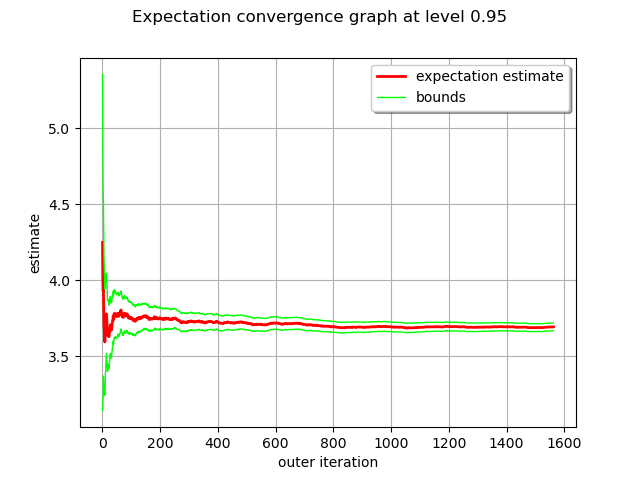
The mean estimate of the metamodel is

print("Mean of the Ishigami metamodel : %.3e" % expectation[0])

Out:

Mean of the Ishigami metamodel : 3.694e+00

We draw the convergence history.

graph = algo.drawExpectationConvergence()
view = otv.View(graph)

For reference, the exact mean of the Ishigami model is :

print("Mean of the Ishigami model : %.3e" % im.expectation)

plt.show()

Out:

Mean of the Ishigami model : 3.500e+00