Generate low discrepancy sequences

In this examples we are going to expose the available low discrepancy sequences in order to approximate some integrals.

The following low-discrepancy sequences are available:

• Sobol

• Faure

• Halton

• reverse Halton

• Haselgrove

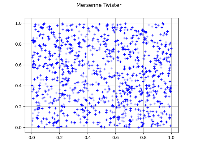
To illustrate these sequences we generate their first 1024 points and compare with the sequence obtained from the pseudo random generator (Merse Twister) as the latter has a higher discrepancy.

from __future__ import print_function
import openturns as ot
import math as m
import openturns.viewer as viewer
from matplotlib import pylab as plt
ot.Log.Show(ot.Log.NONE)

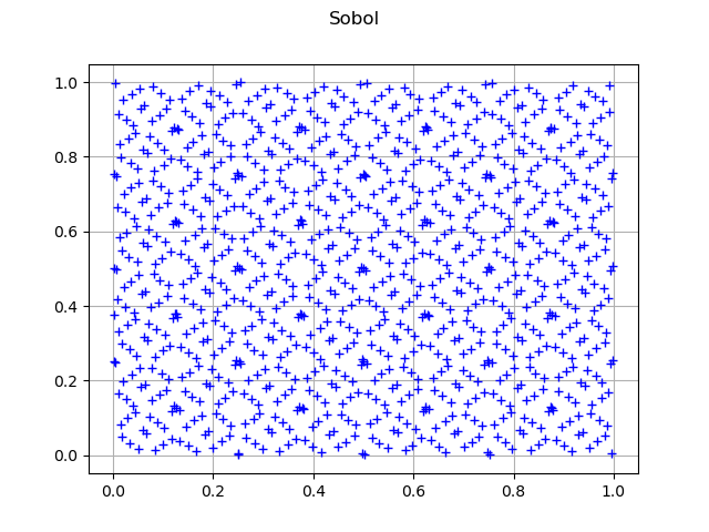
1. Sobol sequence

dimension = 2
size = 1024
sequence = ot.SobolSequence(dimension)
sample = sequence.generate(size)
graph = ot.Graph("Sobol", "", "", True, "")
cloud = ot.Cloud(sample)
graph.add(cloud)
view = viewer.View(graph)

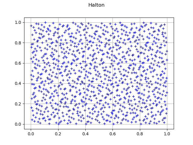
2. Halton sequence

dimension = 2
sequence = ot.HaltonSequence(dimension)
sample = sequence.generate(size)
graph = ot.Graph("Halton", "", "", True, "")
cloud = ot.Cloud(sample)
graph.add(cloud)
view = viewer.View(graph)

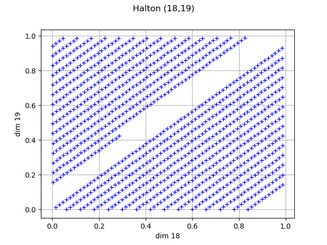
3. Halton sequence in high dimension: bad filling in upper dimensions

dimension = 20
sequence = ot.HaltonSequence(dimension)
sample = sequence.generate(size).getMarginal([dimension-2, dimension-1])
graph = ot.Graph("Halton (" + str(dimension - 2) + "," + str(dimension-1) + ")",
                 "dim " + str(dimension-2), "dim " + str(dimension-1), True, "")
cloud = ot.Cloud(sample)
graph.add(cloud)
view = viewer.View(graph)

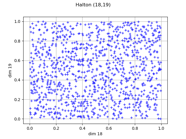
4. Scrambled Halton sequence in high dimension

dimension = 20
sequence = ot.HaltonSequence(dimension)
sequence.setScrambling("RANDOM")
sample = sequence.generate(size).getMarginal([dimension-2, dimension-1])
graph = ot.Graph("Halton (" + str(dimension - 2) + "," + str(dimension-1) + ")",
                 "dim " + str(dimension-2), "dim " + str(dimension-1), True, "")
cloud = ot.Cloud(sample)
graph.add(cloud)
view = viewer.View(graph)

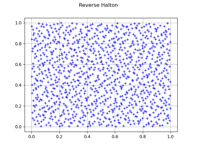
5. Reverse Halton sequence

dimension = 2
sequence = ot.ReverseHaltonSequence(dimension)
sample = sequence.generate(size)
print('discrepancy=',
      ot.LowDiscrepancySequenceImplementation.ComputeStarDiscrepancy(sample))
graph = ot.Graph("Reverse Halton", "", "", True, "")
cloud = ot.Cloud(sample)
graph.add(cloud)
view = viewer.View(graph)

Out:

discrepancy= 0.0035074981424325635

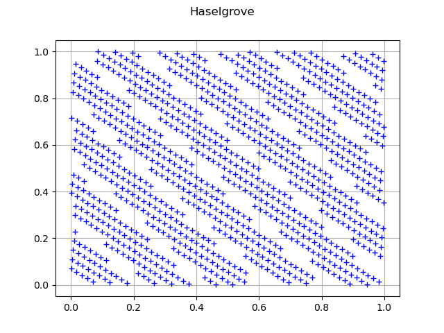
6. Haselgrove sequence

dimension = 2
sequence = ot.HaselgroveSequence(dimension)
sample = sequence.generate(size)
graph = ot.Graph("Haselgrove", "", "", True, "")
cloud = ot.Cloud(sample)
graph.add(cloud)
view = viewer.View(graph)

Compare with uniform random sequence

distribution = ot.ComposedDistribution([ot.Uniform(0.0, 1.0)]*2)
sample = distribution.getSample(size)
print('discrepancy=',
      ot.LowDiscrepancySequenceImplementation.ComputeStarDiscrepancy(sample))
graph = ot.Graph("Mersenne Twister", "", "", True, "")
cloud = ot.Cloud(sample)
graph.add(cloud)
view = viewer.View(graph)
plt.show()

Out:

discrepancy= 0.03623785775796684