Logistic growth model

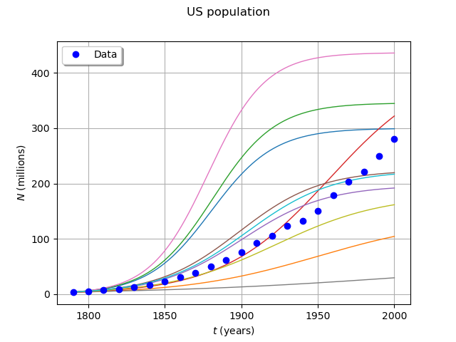
In this example, we use the logistic growth model in order to show how to define a function which has a vector input and a field output. We use the OpenTURNSPythonPointToFieldFunction class to define the derived class and its methods.

Define the model

from openturns.usecases import logistic_model
import openturns as ot
import openturns.viewer as viewer
from matplotlib import pylab as plt

ot.Log.Show(ot.Log.NONE)

We load the logistic model from the usecases module :

lm = logistic_model.LogisticModel()

We get the data from the LogisticModel data class (22 dates with population) :

ustime = lm.data.getMarginal(0)
uspop = lm.data.getMarginal(1)

We get the input parameters distribution distX :

distX = lm.distX

We define the model :

class Popu(ot.OpenTURNSPythonPointToFieldFunction):
    def __init__(self, t0=1790.0, tfinal=2000.0, nt=1000):
        grid = ot.RegularGrid(t0, (tfinal - t0) / (nt - 1), nt)
        super(Popu, self).__init__(3, grid, 1)
        self.setInputDescription(["y0", "a", "b"])
        self.setOutputDescription(["N"])
        self.ticks_ = [t[0] for t in grid.getVertices()]
        self.phi_ = ot.SymbolicFunction(["t", "y", "a", "b"], ["a*y - b*y^2"])

    def _exec(self, X):
        y0 = X[0]
        a = X[1]
        b = X[2]
        phi_ab = ot.ParametricFunction(self.phi_, [2, 3], [a, b])
        phi_t = ot.ParametricFunction(phi_ab, [0], [0.0])
        solver = ot.RungeKutta(phi_t)
        initialState = [y0]
        values = solver.solve(initialState, self.ticks_)
        return values * [1.0e-6]


F = Popu(1790.0, 2000.0, 1000)
popu = ot.PointToFieldFunction(F)

Generate a sample from the model

Sample from the model

size = 10
inputSample = distX.getSample(size)
outputSample = popu(inputSample)

ot.ResourceMap.SetAsUnsignedInteger("Drawable-DefaultPalettePhase", size)

Draw some curves

graph = outputSample.drawMarginal(0)
graph.setTitle("US population")
graph.setXTitle(r"$t$ (years)")
graph.setYTitle(r"$N$ (millions)")
cloud = ot.Cloud(ustime, uspop)
cloud.setPointStyle("circle")
cloud.setLegend("Data")
graph.add(cloud)
graph.setLegendPosition("topleft")
view = viewer.View(graph)
plt.show()